---
title: "The Brighton Secondary School System"
subtitle: "A strategic view"
author: "Adam Dennett, UCL Centre for Advanced Spatial Analysis"
date: today
abstract: |
Brighton & Hove is deciding what to do about a secondary school system
that is losing children faster than it is losing places. This document
assembles what can be established about that system from published
data alone: where the schools and the children are, how reachable the
schools actually are by bus, how demand has moved over sixteen years,
and what a model of the whole system says about the choices in front
of the council. It is written to be argued with.
---
::: {.callout-tip appearance="default" icon="true"}
## Try the options yourself
Everything in this document comes out of one model, and that model runs in a
browser. **[Open the school places simulator](https://adamdennett-bh-school-system.share.connect.posit.cloud/){target="_blank"}**
to change admission numbers, catchments, Longhill's site or the
oversubscription priorities, and watch what happens to each school's intake,
to journey times, to the mix of pupils and to school budgets.
There is also [a guide to the model, stage by
stage](model-guide.qmd), for anyone who wants to check how it works.
:::
::: {.callout-warning appearance="default" icon="true"}
## Beta
**This simulator is currently in beta test mode** - outputs have not been validated fully, so nothing should, at this point, be taken as reliable, however the simulator shows what could be possible to develop and outputs that are possible.
:::
```{r setup}
#| include: false
source(here::here("R", "00_core.R"))
library(scales)
library(patchwork)
knitr::opts_chunk$set(dev = "ragg_png", dpi = 150)
# ---- Everything the document draws on --------------------------------
oi <- bh_data("open_inputs.rds")
acc <- bh_data("accessibility.rds")
# deprivation_open.rds is not loaded here. The document does not read it
# directly - R/02_accessibility.R and R/03_flow_regions.R do, and it
# reaches these pages through what they build. The sources appendix
# checks that claim rather than asserting it.
brt <- bh_data("brightopia.rds")
env <- bh_data("sensitivity_envelope.rds")
perf <- bh_data("performance_panel.rds")
lsoa <- bh_data("lsoa.geojson")
catch <- bh_data("catchments_current.geojson") %>% st_transform(4326)
# Loaded here as well as in the sections that use them, so the executive
# summary can quote figures that are computed further down the document.
rc <- bh_data("reception_cohort.rds")
os <- bh_data("open_scenarios.rds")
conv <- bh_data("adjudicator_conversion.rds")
fp <- bh_data("factsheet_panel.rds")
# Section 6 builds on this, and the executive summary quotes it before
# section 6 runs, so it is loaded here with everything else.
sfin <- bh_data("school_finance.rds")
fmt_n <- function(x, d = 0) formatC(round(x, d), big.mark = ",", format = "f", digits = d)
fmt_pct <- function(x, d = 0) paste0(formatC(x, format = "f", digits = d), "%")
```
```{r choice-fits}
#| include: false
# Section 5.4 asks which published number families respond to. Those
# fits are built here, once, because the executive summary and section 9
# both quote them before that section runs -- and because computing the
# same relationship twice is how this document previously came to report
# two different R-squared values for it.
#
# The specification, fixed in one place:
#
# response log(preferences per place). It is a positive ratio and
# the effect is multiplicative: a point of Attainment 8
# moves demand by a percentage, not by a fixed number of
# applications. This is the specification the open model's
# own choice regression uses.
# predictor the score, entered linearly, as in section 2.3.
# window a five-year mean -- the same window as the attractiveness
# weighting in section 4.5, so the two agree.
#
# The open model publishes the same regression fitted to the single 2024
# round (os$choice_tbl). That is left as it is; the two differ, and
# section 5.4 says by how much and why.
DECAY_A <- acc$pref$decay
PREF_WIN <- 5
ch_hi <- max(fp$factsheets$year)
ch_lo <- ch_hi - PREF_WIN + 1
ch_prefs <- fp$factsheets %>%
filter(name != "Total", year >= ch_lo) %>%
group_by(name) %>%
summarise(p1 = mean(pref1), p2 = mean(pref2), p3 = mean(pref3),
.groups = "drop") %>%
# The factsheets say "Hove Park School" and the performance tables
# "Hove Park School and Sixth Form Centre", so the join goes by URN.
inner_join(oi$attract %>% select(urn, name), by = "name")
stopifnot(nrow(ch_prefs) == 10)
CH_MEASURES <- c("Weighted (ranks 1-3)", "First preferences",
"Second preferences", "Third preferences",
"M5 attractiveness")
CH_BUTTONS <- c("Weighted", "First", "Second", "Third", "M5")
CH_DEFAULT <- "Weighted (ranks 1-3)"
# The full model's attractiveness (section 7.6): balanced so that, once
# distance, the catchment term and competition have done their work, the
# model's demand for each school matches its share of first preferences.
# It is what the simulator's sliders multiply. On a city mean of one, so
# it sits on the same log axis as the preference measures.
mt <- bh_data("model_terms.rds")
ch_w5 <- mt$calibrated$W / mean(mt$calibrated$W)
cd <- os$choice %>%
select(urn, school, pan, att8, va) %>%
inner_join(ch_prefs %>% select(-name), by = "urn") %>%
mutate(short = str_remove(school,
" (School|High School|Community Academy|Catholic School).*"),
`Weighted (ranks 1-3)` = (p1 + DECAY_A * p2 + DECAY_A^2 * p3) / pan,
`First preferences` = p1 / pan,
`Second preferences` = p2 / pan,
`Third preferences` = p3 / pan,
`M5 attractiveness` = unname(ch_w5[oi$attract$name[match(urn, oi$attract$urn)]]))
# All four measures must be strictly positive, or the log response fails.
stopifnot(nrow(cd) == 10, min(as.matrix(cd[CH_MEASURES])) > 0)
CH_PRED <- c(att8 = "Attainment 8 (headline)",
va = "Value added (Lever report)")
CH_COL <- c(att8 = "#b2182b", va = "#2166ac")
ch_fit <- function(x, y) {
m <- lm(log(y) ~ x)
xs <- seq(min(x), max(x), length.out = 60)
list(x = xs, y = exp(coef(m)[[1]] + coef(m)[[2]] * xs),
r2 = summary(m)$r.squared, slope = coef(m)[[2]])
}
CH_FITS <- expand.grid(measure = CH_MEASURES, pred = names(CH_PRED),
stringsAsFactors = FALSE) %>%
mutate(f = map2(measure, pred, ~ ch_fit(cd[[.y]], cd[[.x]])),
r2 = map_dbl(f, "r2"))
ch_one <- function(m, p) CH_FITS$f[[which(CH_FITS$measure == m &
CH_FITS$pred == p)]]
ch_r2 <- function(m, p) ch_one(m, p)$r2
# Does knowing the school's contribution add anything once its headline
# score is already in the model? Fitted on the default measure.
ch_combined <- lm(log(cd[[CH_DEFAULT]]) ~ att8 + va, data = cd)
ch_combined_r2 <- summary(ch_combined)$r.squared
ch_combined_va <- coef(ch_combined)[["va"]]
# M5's attractiveness: is the log scale the right one, does one school
# carry it, and how much do the two faith schools - which have no
# catchment term to carry their demand - drive it?
ch_w5_lin <- summary(lm(`M5 attractiveness` ~ att8, data = cd))$r.squared
ch_w5_slope <- ch_one("M5 attractiveness", "att8")$slope
ch_w5_loo <- vapply(seq_len(nrow(cd)), function(i)
summary(lm(log(`M5 attractiveness`) ~ att8, data = cd[-i, ]))$r.squared,
numeric(1))
ch_w5_8 <- summary(lm(log(`M5 attractiveness`) ~ att8,
data = cd %>% filter(!urn %in% oi$schools$urn[oi$schools$faith])))$r.squared
ch_w5_of <- function(s) cd$`M5 attractiveness`[cd$short == s]
# Which admissions round the open model's own regression is fitted to.
# Derived rather than assumed: its first-preference counts match exactly
# one year of the factsheet panel, and the answer is not the latest one.
ch_open_year <- fp$factsheets %>%
filter(name != "Total") %>%
select(name, year, pref1) %>%
inner_join(oi$attract %>% select(urn, name), by = "name") %>%
inner_join(os$choice %>% select(urn, first_pref), by = "urn") %>%
group_by(year) %>%
summarise(all_match = all(pref1 == first_pref), n = n(), .groups = "drop") %>%
filter(all_match, n == nrow(cd)) %>%
pull(year)
stopifnot(length(ch_open_year) == 1)
ch_open_r2 <- function(s) os$choice_tbl$r2[os$choice_tbl$spec == s]
# The open model now fits this same regression on this same weighted
# measure, and publishes it. The two used to disagree, because the same
# relationship was being computed twice; this asserts that they no
# longer do, so a future change to either side fails the render instead
# of quietly producing two different numbers for one thing.
stopifnot(
abs(ch_r2(CH_DEFAULT, "att8") -
ch_open_r2("Attainment 8, weighted preferences")) < 5e-3,
abs(ch_r2(CH_DEFAULT, "va") -
ch_open_r2("Value-added, weighted preferences")) < 5e-3,
abs(ch_combined_r2 -
ch_open_r2("Attainment 8 + value-added, weighted preferences")) < 5e-3)
# The negative value-added coefficient the open model reports on the
# single round, kept so section 5.4 can say what it was.
ch_one_round_va <- {
m <- os$choice_models[["Attainment 8 + value-added"]]
coef(m)[["va"]]
}
```
```{r exec-figures}
#| include: false
# Headline figures for the executive summary. Every one of these is
# recomputed in the section it belongs to; they are gathered here only
# so the summary can quote them before those sections run.
ex_now <- rc$secondary_city %>% slice_max(year, n = 1)
ex_peak <- rc$secondary_city %>% slice_max(y7_offers, n = 1)
ex_proj <- rc$projection %>% slice_max(entry_year, n = 1)
ex_fall <- 100 * (ex_proj$central - ex_now$y7_offers) / ex_now$y7_offers
ex_places <- sum(oi$schools$pan2026[oi$schools$name != "Peacehaven Community School"])
ex_surplus <- ex_places - ex_proj$central
ex_zero30 <- acc$lsoa %>% filter(places_30 < 1)
ex_corner <- acc$worst_corner
ex_rat <- conv$conv %>%
group_by(school) %>%
summarise(rate = sum(p1_offered) / sum(p1_named), .groups = "drop")
ex_open <- sum(ex_rat$rate > 0.999)
# The weighted measure, which is what section 5.4 shows by default.
ex_r2_att8 <- ch_r2(CH_DEFAULT, "att8")
ex_r2_va <- ch_r2(CH_DEFAULT, "va")
# How strongly demand follows the headline score, and where the two
# schools serving the most disadvantaged intakes sit on each measure.
ex_att8_pct <- 100 * (exp(ch_one(CH_DEFAULT, "att8")$slope) - 1)
ex_cd <- cd %>% mutate(r_att8 = rank(-att8), r_va = rank(-va))
ex_cd_of <- function(s, col) ex_cd[[col]][ex_cd$short == s]
# Same specification as section 2.3, which follows the Lever report:
# log outcome, logged rates, KS2 score entered linearly.
ex_nat <- perf$national %>%
filter(!is.na(ATT8SCR), ATT8SCR > 0) %>%
mutate(ks2_c = KS2ASS - 100)
ex_fsm <- summary(lm(log(ATT8SCR) ~ log(PTFSM6CLA1A), data = ex_nat))$r.squared
ex_prior <- summary(lm(log(ATT8SCR) ~ ks2_c, data = ex_nat))$r.squared
ex_absn <- summary(lm(log(ATT8SCR) ~ log(PERCTOT), data = ex_nat))$r.squared
ex_lh <- brt$at_original_beta %>%
filter(str_detect(name, "Longhill")) %>%
mutate(fill_2026 = modelled / pan2026, fill_2024 = modelled / pan2024)
# The between-school share of *pupil-level* variance. This cannot be
# computed from school-level aggregates - it needs pupil records - so it
# is quoted from the school-effectiveness literature, not estimated
# here. Defined at the top because both the executive summary and
# section 2.4 use it.
SCHOOL_LO <- 8; SCHOOL_HI <- 15
# Variance decomposition from the Lever model, for the summary. Section
# 2.4 recomputes these from the same object.
ex_sed <- bh_data("school_effect_decomp.rds")
.pick <- function(d, pat) d[["Share of total %"]][grepl(pat, d$Component)][1]
ex_wf_all <- .pick(ex_sed$decomp_all, "^Endogenous")
ex_ex_all <- .pick(ex_sed$decomp_all, "^Exogenous")
ex_wf_dis <- .pick(ex_sed$decomp_dis, "^Endogenous")
# The share a school can actually reach: workforce plus the
# school-controllable half of absence. Section 2.5 derives this.
ex_lev <- bh_data("school_leverage.rds")$leverage
ex_reach <- ex_lev$reachable[ex_lev$who == "All pupils"]
ex_abs_school <- ex_lev$absence_school[ex_lev$who == "All pupils"]
# Recomputed from the fitted model rather than the cached table, so that
# workforce + school-reachable absence actually sums to the reachable
# total quoted alongside it. It differs from the cached 3.3% by under a
# percentage point; section 2.5 explains why.
ex_wf_recomp <- ex_lev$workforce[ex_lev$who == "All pupils"]
```
::: {.callout-note appearance="simple"}
## No pupil-level data is used here
No pupil-level record is used anywhere in this document. Almost every
figure comes from data the council, the DfE or the ONS has already
published, or from a model built on top of it. The one exception is a
table the council gave the Schools Adjudicator in the 2026/27 case: how
many first, second and third preferences each catchment's children gave
each school, over three rounds (item 8.1 of its evidence). It was
received as a party to that case rather than published; it is aggregated
to catchment and identifies no one; and the full model in section 7 is
calibrated to it (@sec-m5). Where a question can only be
answered with data the council holds but has not released, that is said
plainly rather than glossed over --- and section 9 lists what those
releases would be.
:::
# Executive summary {#sec-exec}
## The situation
Brighton & Hove has a secondary school system built for more children
than it now has, and the shortfall is going to get worse before anything
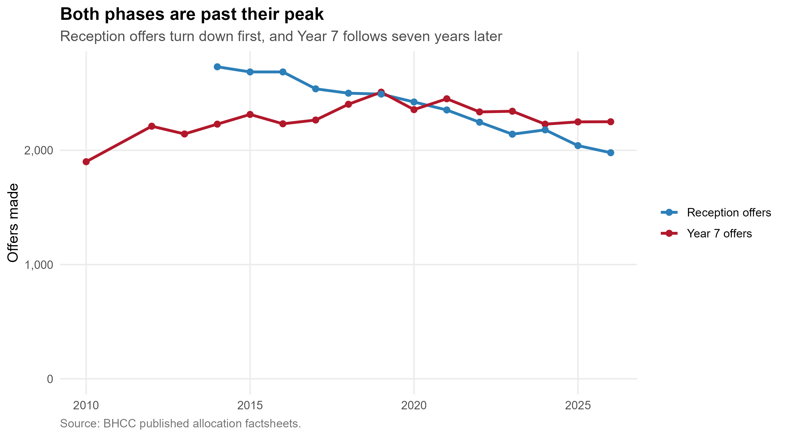
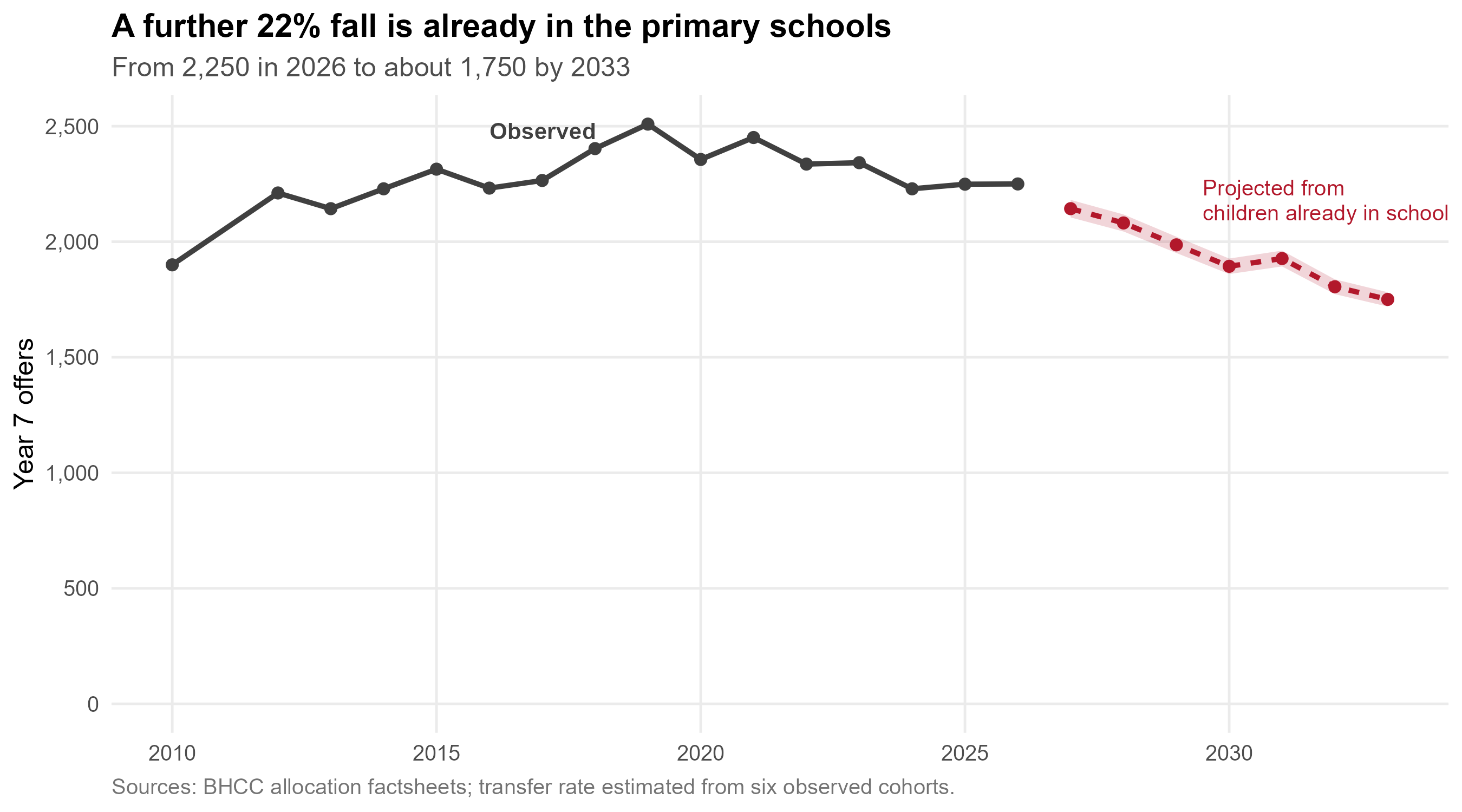
the council decides can affect it. Year 7 offers peaked at
`r fmt_n(ex_peak$y7_offers)` in `r ex_peak$year` and stood at
`r fmt_n(ex_now$y7_offers)` in `r ex_now$year`. The children who will
enter Year 7 in `r ex_proj$entry_year` are already in the city's primary
schools, and there are about **`r fmt_n(ex_proj$central)`** of them ---
a further fall of `r fmt_pct(abs(ex_fall), 0)`. Against roughly
`r fmt_n(ex_places)` published places, that implies something like
**`r fmt_n(ex_surplus)` surplus places**, or two and a half average
secondary schools' worth.
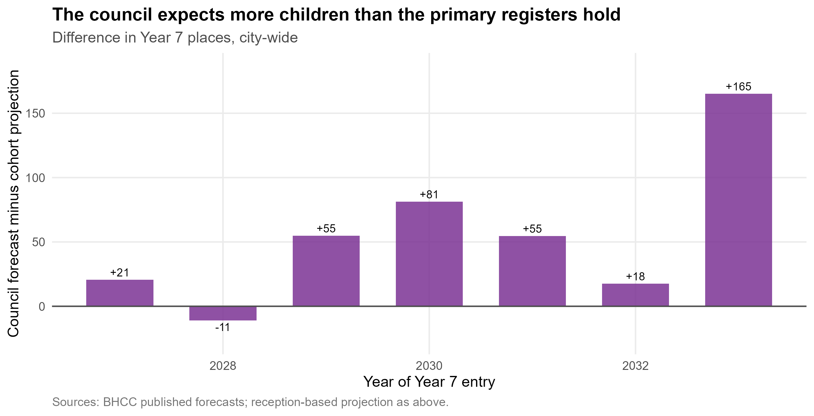
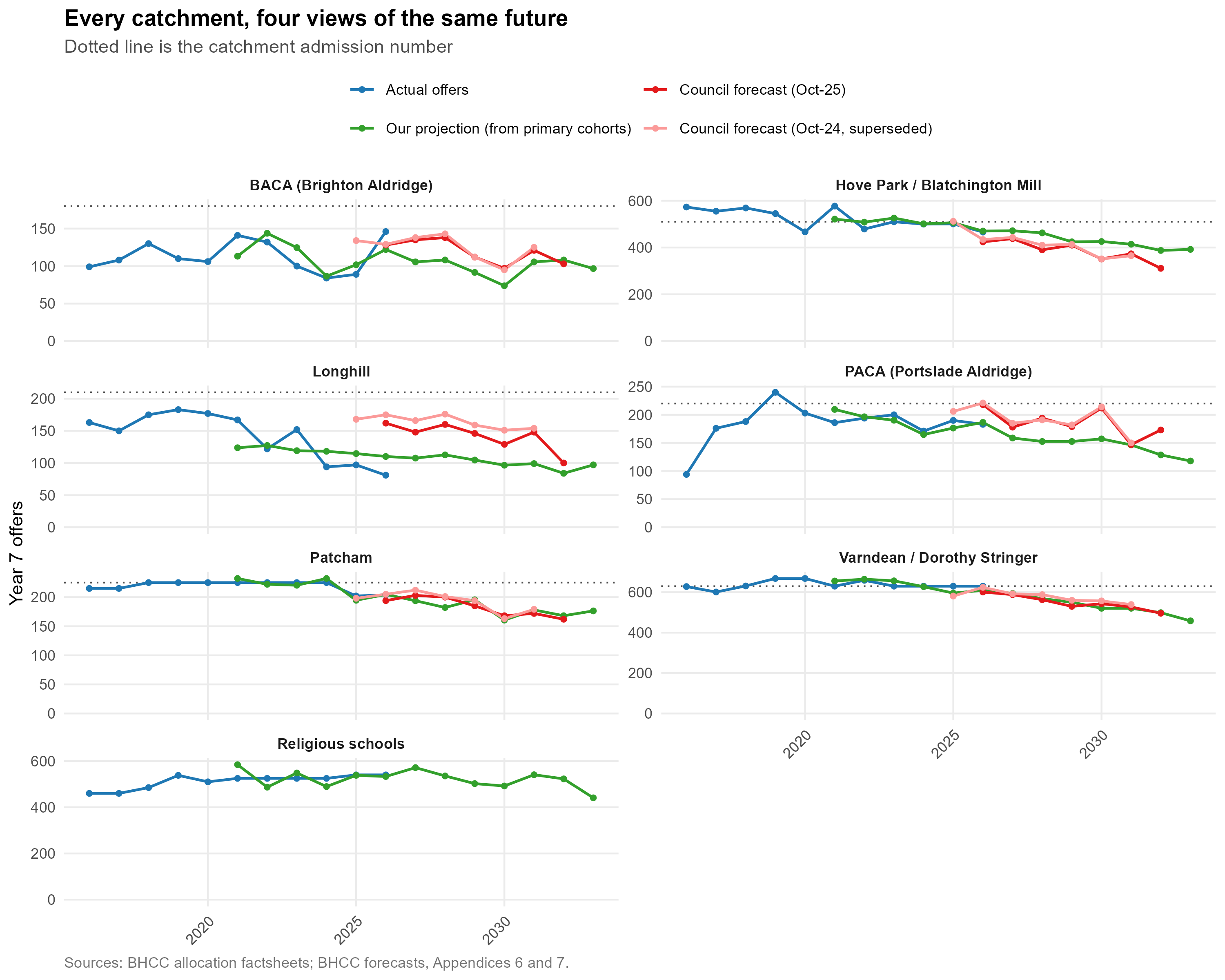
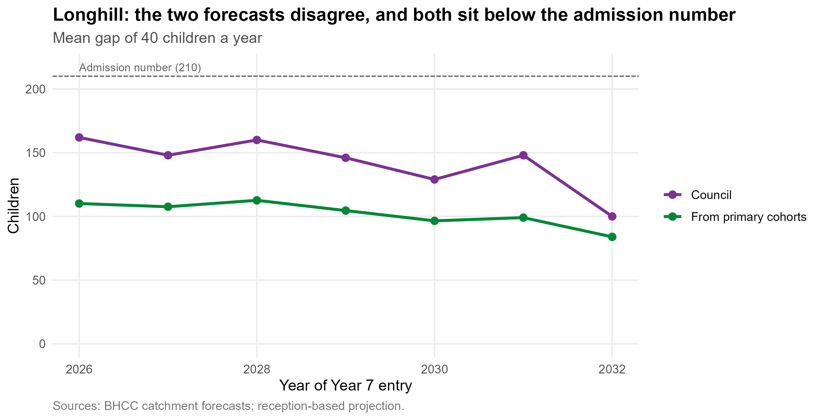
The council's own catchment forecasts sit above that projection in
almost every year, and the gap is widest in the Longhill catchment ---
the place where the consequences of being wrong are largest.
```{r exec-va}
#| include: false
ex_vac <- bh_data("value_added_choice.rds")
ex_va_sch <- function(s, col) {
d <- ex_vac$schools[ex_vac$schools$year == 2026, ]
d[[col]][d$short == s]
}
ex_va_even <- ex_vac$even[ex_vac$even$year == 2026, ]
ex_va_city <- function(b, col)
ex_vac$city[[col]][ex_vac$city$year == 2026 & ex_vac$city$basis == b]
```
## What the evidence says
**This is not a school quality problem.** Across English secondaries,
absence explains `r fmt_pct(100 * ex_absn, 0)` of the variation in
Attainment 8 and prior attainment `r fmt_pct(100 * ex_prior, 0)`, while
deprivation explains only `r fmt_pct(100 * ex_fsm, 0)`. Once intake is
accounted for, Brighton's schools mostly perform above what their intake
predicts. The largest lever available to the city is **absence**, not
social mixing --- established in detail in
[How to Pull the Right Lever](https://adamdennett.github.io/school_attainment_tool/index.html).
**Moving children between schools is a weak instrument, and this is the
single most important point for admissions policy.** Decomposing the
variance in Attainment 8 shows that a school can reach about
**`r fmt_pct(ex_reach, 0)`** of what separates its results from another's
--- consistent with sixty years of school-effectiveness research. The
rest arrives with the children. Crucially, **almost all of that reachable
share runs through attendance**: the workforce a school hires accounts
for only `r fmt_pct(ex_wf_recomp, 1)`, while the school-controllable half
of absence accounts for `r fmt_pct(ex_abs_school, 0)`. Redistribution touches
neither. It changes which building a child attends without changing their
attendance or their circumstances. This is not an argument that schools
do not matter --- it is an argument that the council's lever is
attendance, and attendance is not an admissions policy.
**For disadvantaged pupils, concentration is not the harm it is assumed
to be.** Nationally, once absence and prior attainment are accounted
for, disadvantaged pupils do slightly *better* in schools with more
disadvantaged pupils, not worse. The effect is small, and it appears to
run through schools organised to serve those pupils rather than through
concentration itself --- but it points the opposite way to the
council's aim of reducing concentrations. Brighton Aldridge is the local
example: about half its pupils are disadvantaged, and its disadvantaged
pupils leave with better GCSE results than comparable pupils elsewhere
in England (@sec-concentration-evidence). So where an option here raises
the segregation index, that counts against it under the council's
policy aim; it is not, on the evidence, a cost to disadvantaged pupils'
results.
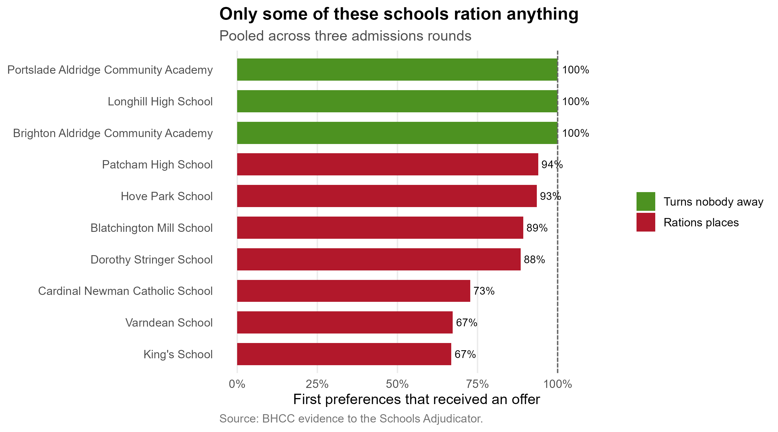
**Admissions criteria only bind at some schools.**
`r ex_open` of the `r nrow(ex_rat)` schools offered a place to every
first-preference applicant. For those schools the catchment rule, the
sibling rule and the free school meals quota do nothing at all. The city
runs two admissions systems under one set of rules, and public argument
about criteria concerns only one of them.
**Families are choosing on the wrong number, and the council's own
advice points them to it.** Its secondary admissions guide tells parents
to look in each school's prospectus for its "National Curriculum test
results, public exam results" and to read its Ofsted reports
([Secondary school admissions guide 2027 to 2028](https://www.brighton-hove.gov.uk/schools-and-learning/school-policies-reports-strategies-and-other-documents/secondary-school-admissions-guide-2027-2028)) ---
raw figures that mostly describe who a school admits. Families do as
they are advised. Headline Attainment 8 explains
`r fmt_pct(100 * ex_r2_att8, 0)` of the variation in how heavily each
school is preferred, and each point of it goes with about
`r sprintf("%.0f", ex_att8_pct)`% more preferences per place. The
value-added measure --- what the school actually contributes ---
explains `r fmt_pct(100 * ex_r2_va, 0)`.
**That advice works against the council's own position.** A school
serving a more disadvantaged intake posts a lower headline score, so it
is chosen less; its intake shrinks and becomes more disadvantaged still;
and its headline score falls again. Brighton Aldridge is last of the ten
on the headline measure and
`r c("first","second","third","fourth","fifth","sixth","seventh","eighth","ninth","tenth")[ex_cd_of("Brighton Aldridge", "r_va")]`
on value added. Longhill's headline score is
`r sprintf("%.0f", max(ex_cd$att8) - ex_cd_of("Longhill", "att8"))` points
below the city's highest, but on value added it is
`r sprintf("%.1f", max(ex_cd$va) - ex_cd_of("Longhill", "va"))` points
below the best --- most of what separates it from the most popular
schools is intake, not teaching. By steering families towards the
headline number, the council lowers the pull of the very school whose
viability it is trying to secure, shrinks the roll its funding depends
on, and concentrates disadvantage in the schools its own guidance makes
least attractive --- the opposite of its stated aim. It is the one part
of the Longhill problem the council could change at no cost
(@sec-choice).
**And it is the largest lever modelled here.** Run the city with families
reading the four-year value-added measure as closely as they now read the
headline score, holding everything else --- same places, same catchments,
same rules --- and the intakes move further than any boundary change in
this document. Brighton Aldridge goes from
`r fmt_n(round(ex_va_sch("Brighton Aldridge", "att8_intake")))` children
to `r fmt_n(round(ex_va_sch("Brighton Aldridge", "va_intake")))` on 180
places, from half empty to
`r sprintf("%.0f%%", 100 * ex_va_sch("Brighton Aldridge", "va_fill"))`
full; Hove Park and Portslade Aldridge fill; mean journeys shorten, and
the extra distance the most deprived children travel falls from
`r sprintf("%.1f", ex_va_city("Attainment 8", "dep_gap"))` to
`r sprintf("%.1f", ex_va_city("Value added", "dep_gap"))` minutes each
way. **The share of the city's empty Year 7 places sitting in just three
schools falls from
`r sprintf("%.0f%%", 100 * ex_va_even$top3_att8)` to
`r sprintf("%.0f%%", 100 * ex_va_even$top3_va)`** --- which is the
difference between a surplus that is a budgeting problem and one that is
a viability problem. It creates no places and removes none: what changes
is which schools are empty (@sec-value-added-choice).
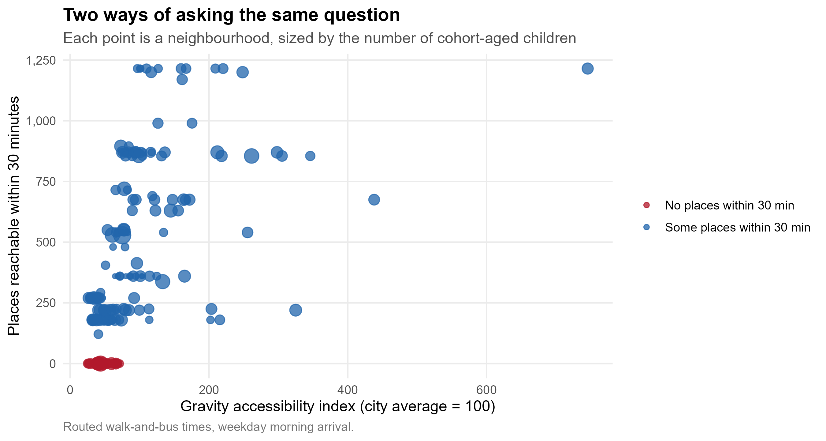
**Physical access is unequal, and unequal in the worst direction.**
`r nrow(ex_zero30)` of `r nrow(acc$lsoa)` neighbourhoods --- about
`r fmt_n(sum(ex_zero30$Oi))` cohort-aged children --- can reach **no**
secondary school place within 30 minutes by walking and bus.
Accessibility and child poverty correlate at
`r sprintf("%.2f", acc$acc_dep_spearman)`: `r nrow(ex_corner)`
neighbourhoods sit in both the least-reachable third and the most
deprived third.
**Longhill has already been shrunk to about what geography supports.**
A model of where children would go if only distance and school size
mattered gives it `r fmt_n(ex_lh$modelled)` children ---
`r fmt_pct(100 * ex_lh$fill_2024, 0)` of its former admission number of
`r fmt_n(ex_lh$pan2024)`, but `r fmt_pct(100 * ex_lh$fill_2026, 0)` of
the reduced `r fmt_n(ex_lh$pan2026)` now in force. The reduction has
already done most of what a reduction can do, and the remaining problem
is a falling cohort against a reserve that supports about
`r sprintf("%.1f", os$years_left)` more years.
**But the money is not a Longhill problem.**
`r sum(sfin$change$res_change < 0)` of the city's
`r nrow(sfin$change)` secondary schools have been spending their
reserves, `r sum(sfin$exposure$reserve_pct < 0)` are now overdrawn, and
the two in the deepest deficit are not Longhill --- they are Hove Park
and Cardinal Newman, one of them the largest and fastest-growing school
in the city. @sec-money sets out every school's position and which of
them the pupil projections put next in line.
## What follows
1. **Decide about Longhill on the financial timetable**, not the
consultation one. The horizon is about
`r sprintf("%.1f", os$years_left)` years.
2. **Treat the instruments as a package.** Moving the school, changing
its admission number and redrawing catchments each fall short alone
and compose when combined. Picking one and waiting is the worst
available option. If the council puts access for disadvantaged
children first, the package should be led by a smaller Longhill at
the top of Elm Grove with the catchments redrawn round it
(@sec-weighing).
3. **Change the admissions guide's advice, and publish a contextualised
measure alongside Attainment 8.** It costs nothing, needs no
consultation, and is the largest single change modelled in this
document: if families read what a school adds rather than the score it
publishes, Brighton Aldridge fills
(`r fmt_n(round(ex_va_sch("Brighton Aldridge", "att8_intake")))` children
to `r fmt_n(round(ex_va_sch("Brighton Aldridge", "va_intake")))` on 180
places), the share of the city's empty places concentrated in three
schools falls from
`r sprintf("%.0f%%", 100 * ex_va_even$top3_att8)` to
`r sprintf("%.0f%%", 100 * ex_va_even$top3_va)`, and deprived children's
extra travel falls by about a minute each way (@sec-value-added-choice).
4. **Treat the bus network as an admissions instrument.** It is the only
lever here that widens choice without taking anything from anyone.
5. **Release ten tables** (§9) that would convert most of the bands in
this document into estimates.
## How confident to be
The demographic findings are the firmest: they are counts of children
already in school, adjusted by a transfer rate that has varied by under
two percentage points in a decade. The accessibility findings are firm
in direction and approximate in magnitude --- modelled journey times,
not measured ones. The model results in sections 7 and 8 are the
softest: the model is swept rather than calibrated, because calibration
needs data the council has not released. Every comparison there is
robust across the swept range; no individual number should be read as a
prediction.
# The secondary school system {#sec-system}
Ten secondary schools serve Brighton & Hove: six community schools run
by the local authority, two academies (Brighton Aldridge and Portslade
Aldridge) and two church schools (King's and Cardinal Newman) that set
their own admissions. An eleventh, Peacehaven Community School, sits
just outside the boundary but inside the travel-to-school geography, and
is included throughout because families on the eastern edge of the city
treat it as a real option.
One of the ten is not a single building. **Hove Park teaches Years 7 and
8 at its Valley Campus on Hangleton Way**, 1.65 km west of the Nevill
Road site its address gives, and moves pupils to Nevill Road in Year 9.
The council gave statutory notice on 8 June 2026 to close the Valley
Campus on 31 August 2028 and bring the school onto one site. Because
this document is about Year 7, every figure here for entry years up to
2027 puts Hove Park at Hangleton Way and every figure from 2028 puts it
at Nevill Road. It makes little difference to how many children the
school takes, and a large difference to which children: at Hangleton Way
it draws about twice as many from Hangleton & Knoll and much less from
Westdene and Poets' Corner
([the model guide](https://adamdennett.github.io/bh-school-system/model-guide.html#sec-cij-hove-park)).
The city allocates places by **catchment area with a lottery tie-break**
for oversubscribed schools --- an arrangement that is very unusual in
England, where distance from the school gate usually decides priority.
It dates from the closure of CoMArt in the east of the city in 2005, and
the catchment system that replaced distance-based allocation in 2008.
CoMArt is marked on the map below because the shape of the system is
still partly the shape of that closure.
## Where the schools, the catchments and the children are {#sec-orientation}
```{r fig-orientation}
#| fig-cap: "Schools, catchment boundaries and the cohort-aged child population. Use the control at the top right to turn each layer on and off."
# ---- Schools ---------------------------------------------------------
sch <- schools_sf(oi$schools)
sch_popup <- sprintf(
"<b>%s</b><br>Admission number 2024: %s<br>Planned 2030: %s%s",
sch$name, sch$pan2024, sch$pan2030,
ifelse(is.na(sch$catchment),
"<br><i>Faith school, admits city-wide</i>",
paste0("<br>Catchment: ", CATCH_LABELS[sch$boundary_catchment])))
# ---- Children per LSOA ----------------------------------------------
# Oi is the cohort-aged child estimate per zone; zones are LSOA x
# catchment, so an LSOA split by a boundary has to be summed back up.
children <- oi$zones %>%
group_by(lsoa) %>%
summarise(children = sum(Oi, na.rm = TRUE), .groups = "drop")
lsoa_pts <- lsoa %>%
left_join(children, by = c("lsoa21cd" = "lsoa")) %>%
filter(!is.na(children), children > 0) %>%
st_point_on_surface() %>%
suppressWarnings()
pt_xy <- st_coordinates(lsoa_pts)
lsoa_pts$lon <- pt_xy[, 1]; lsoa_pts$lat <- pt_xy[, 2]
# Radius on the square root of the count, so circle *area* is
# proportional to the number of children rather than the radius being -
# the latter exaggerates big areas by a factor of the count.
r_scale <- function(n) 3 + 17 * sqrt(n / max(n, na.rm = TRUE))
pal_catch <- colorFactor(unname(CATCH_COLOURS), names(CATCH_COLOURS))
m <- leaflet(width = "100%", height = 620) %>%
add_basemap() %>%
setView(lng = -0.10, lat = 50.84, zoom = 12) %>%
addPolygons(
data = catch, group = "Catchments",
fillColor = ~pal_catch(catchment), fillOpacity = 0.13,
color = ~pal_catch(catchment), weight = 2.5, opacity = 0.85,
label = ~unname(CATCH_LABELS[catchment]),
highlightOptions = highlightOptions(weight = 4, fillOpacity = 0.25,
bringToFront = FALSE)) %>%
addCircleMarkers(
data = lsoa_pts, lng = ~lon, lat = ~lat, group = "Children",
radius = ~r_scale(children),
fillColor = "#1f4e79", fillOpacity = 0.35,
color = "#1f4e79", weight = 1, opacity = 0.55,
label = ~sprintf("%s: about %s children in the cohort",
lsoa21nm, round(children)))
m <- add_school_layer(m, sch, group = "Schools", popup = sch_popup)
# CoMArt, closed 2005
m <- m %>% addCircleMarkers(
lng = COMART$lon, lat = COMART$lat, group = "CoMArt (closed 2005)",
radius = 6, fillColor = "#b2182b", fillOpacity = 0.9,
color = "white", weight = 2,
popup = "<b>CoMArt</b><br>Closed 2005. Its closure is why the city moved to catchments with a lottery tie-break.",
label = COMART$name)
ic <- logo_icon(COMART$logo)
if (!is.null(ic))
m <- m %>% addMarkers(lng = COMART$lon, lat = COMART$lat, icon = ic,
group = "CoMArt (closed 2005)",
label = COMART$name)
legend_html <- paste0(
'<div style="background:white;padding:8px 12px;border-radius:4px;',
'box-shadow:0 1px 5px rgba(0,0,0,.3);font-family:sans-serif;font-size:12px;line-height:1.6">',
'<div style="font-weight:bold;margin-bottom:4px">Catchment areas, 2025/26</div>',
paste0('<div style="display:flex;align-items:center;gap:6px">',
'<span style="display:inline-block;width:14px;height:14px;background:',
unname(CATCH_COLOURS), ';border-radius:2px;flex-shrink:0"></span><span>',
unname(CATCH_LABELS), '</span></div>', collapse = ''),
'<div style="margin-top:6px;padding-top:6px;border-top:1px solid #ddd">',
'<span style="display:inline-block;width:14px;height:14px;background:#1f4e79;',
'opacity:.35;border-radius:50%;margin-right:6px"></span>Children per LSOA',
' <span style="color:#777">(area ∝ count)</span></div></div>')
m %>%
addLayersControl(
overlayGroups = c("Catchments", "Schools", "Children", "CoMArt (closed 2005)"),
options = layersControlOptions(collapsed = FALSE)) %>%
hideGroup("CoMArt (closed 2005)") %>%
addControl(html = legend_html, position = "bottomright")
```
Three things are worth noticing on that map before any analysis begins.
**The catchments are not equivalent objects.** Four of them contain a
single school; two contain a pair. A child in the Varndean / Dorothy
Stringer or Hove Park / Blatchington Mill catchment has two schools to
name and a realistic chance of one of them. A child in the Longhill,
Patcham, BACA or PACA catchment has one. That asymmetry does more work
in this system than almost anything else, and section 5 returns to it.
**The children are not spread evenly.** The cohort is concentrated in
the centre and west; the east of the city, which contains Longhill's
entire catchment, is thin. Longhill's problem is visible on this map
before any model is run.
**Two schools sit outside the geography entirely.** King's and Cardinal
Newman admit city-wide on faith criteria. Together they hold
`r fmt_n(sum(oi$schools$pan2026[is.na(oi$schools$catchment)]))` places,
about
`r fmt_pct(100 * sum(oi$schools$pan2026[is.na(oi$schools$catchment)]) / sum(oi$schools$pan2026[oi$schools$name != "Peacehaven Community School"]))`
of the city total. Any statement about what catchments do has to be read
against that.
## Where the children actually are {#sec-child-density}
The circles on the map above are LSOA totals, and an LSOA is a blunt
unit --- about 1,500 people, drawn for administrative convenience rather
than to describe a neighbourhood. Two finer views of the same population
follow. They are shown side by side because they answer slightly
different questions, and it is worth deciding which one this document
should carry.
```{r pcd-data}
#| include: false
pcd <- bh_data("postcode_children.csv") %>%
filter(!is.na(easting), !is.na(northing), children > 0)
# Land mask: the union of the city's LSOAs. Without it a smoothed
# surface runs cheerfully out into the Channel.
city <- lsoa %>%
filter(lsoa21cd %in% unique(pcd$lsoa)) %>%
st_transform(27700) %>%
st_union() %>%
st_make_valid()
```
::: {.panel-tabset}
### Density surface
```{r fig-child-density}
#| fig-cap: "Children aged 0-18 per hectare, smoothed from postcode-level estimates with a 400 m kernel and clipped to the built-up area. Census 2021 household composition apportioned to postcode centroids."
BW <- 400 # kernel bandwidth in metres - a walkable neighbourhood
GRID <- 320 # grid resolution
# A weighted kernel density: each child contributes one point, so the
# surface is the density of children rather than of postcodes. Counts are
# apportioned estimates and so fractional; rounding for replication
# changes the total by well under a percent.
reps <- round(pcd$children)
kx <- rep(pcd$easting, reps)
ky <- rep(pcd$northing, reps)
bb <- st_bbox(city)
k <- MASS::kde2d(kx, ky, h = c(BW, BW), n = GRID,
lims = c(bb["xmin"] - 500, bb["xmax"] + 500,
bb["ymin"] - 500, bb["ymax"] + 500))
# kde2d integrates to 1 over square metres. Scale to children per
# hectare so the legend means something to a reader.
dens <- k$z * sum(reps) * 1e4
brks <- c(0, 2, 5, 10, 15, 22, 30, max(45, ceiling(max(dens))))
pal_d <- viridisLite::viridis(length(brks) - 1, option = "magma",
direction = -1, begin = 0.08)
# isoband wants z indexed [y, x]; kde2d returns [x, y].
bands <- isoband::isobands(x = k$x, y = k$y, z = t(dens),
levels_low = brks[-length(brks)],
levels_high = brks[-1])
band_sf <- st_sf(
lo = brks[-length(brks)], hi = brks[-1],
geometry = st_sfc(isoband::iso_to_sfg(bands), crs = 27700)) %>%
st_make_valid() %>%
st_intersection(city) %>%
filter(!st_is_empty(geometry)) %>%
# Simplify while still in metres. Contour bands off a 320 x 320 grid
# carry far more vertices than a screen can show; 15 m is invisible at
# any zoom this map offers and cuts the embedded geometry sharply.
# This has to happen before the transform - in 4326 the tolerance
# would be read as degrees and flatten the whole surface.
st_simplify(dTolerance = 15, preserveTopology = TRUE) %>%
st_transform(4326)
band_sf$col <- pal_d[seq_len(nrow(band_sf))]
band_sf$lab <- sprintf("%g - %g children per hectare", band_sf$lo, band_sf$hi)
leaflet(width = "100%", height = 600,
options = leafletOptions(preferCanvas = TRUE)) %>%
add_basemap() %>%
addPolygons(data = band_sf, fillColor = ~col, fillOpacity = 0.72,
color = NA, weight = 0, label = ~lab, group = "Children") %>%
addPolygons(data = catch, fill = FALSE, color = "#333333",
weight = 1.6, opacity = 0.7, group = "Catchments",
label = ~unname(CATCH_LABELS[catchment])) %>%
add_school_layer(sch, group = "Schools", popup = sch_popup) %>%
addLayersControl(overlayGroups = c("Children", "Catchments", "Schools"),
options = layersControlOptions(collapsed = TRUE)) %>%
addLegend(colors = band_sf$col, labels = band_sf$lab,
title = "Children 0-18<br>per hectare",
position = "bottomright", opacity = 0.8)
```
### Postcode detail
```{r fig-pcd-dots}
#| fig-cap: "Every residential postcode in the city, sized by the number of children aged 0-18 and coloured by income deprivation affecting children. Decile 1 is the most deprived tenth of neighbourhoods nationally."
pcd_sf <- pcd %>%
st_as_sf(coords = c("easting", "northing"), crs = 27700) %>%
st_transform(4326) %>%
filter(!is.na(idaci_decile))
pal_idaci <- colorFactor("RdYlBu", domain = sort(unique(pcd_sf$idaci_decile)))
# Radius on the square root of the count so circle area is proportional
# to children. Scaled well down from the LSOA circles in 2.1: there are
# 4,229 postcodes against 179 LSOAs, so the same per-circle size would
# cover the city in a single wash of ink. The median postcode draws at
# about 3.5 px and the largest at about 9.
#
# preferCanvas matters here rather than being a nicety. Leaflet's
# default renderer gives every marker its own SVG element, and four
# thousand of them is enough to hang or crash a browser tab. On canvas
# they are drawn into a single element and the map stays responsive.
leaflet(width = "100%", height = 600,
options = leafletOptions(preferCanvas = TRUE)) %>%
add_basemap() %>%
addPolygons(data = catch, fill = FALSE, color = "#333333",
weight = 1.6, opacity = 0.7, group = "Catchments",
label = ~unname(CATCH_LABELS[catchment])) %>%
addCircleMarkers(
data = pcd_sf, group = "Postcodes",
radius = ~0.5 + sqrt(children),
fillColor = ~pal_idaci(idaci_decile), fillOpacity = 0.6,
stroke = FALSE,
label = ~sprintf("%s | %.0f children 0-18 | IDACI decile %s",
postcode, children, idaci_decile)) %>%
add_school_layer(sch, group = "Schools", popup = sch_popup) %>%
addLayersControl(overlayGroups = c("Postcodes", "Catchments", "Schools"),
options = layersControlOptions(collapsed = TRUE)) %>%
addLegend(pal = pal_idaci, values = sort(unique(pcd_sf$idaci_decile)),
title = "IDACI decile<br><span style='font-weight:normal'>1 = most deprived</span>",
position = "bottomright", opacity = 0.9)
```
:::
```{r density-check}
#| include: false
# Sanity check on the surface. The comparison has to be like for like:
# the surface is children per hectare, so testing it against the raw
# count in each postcode mostly measures how much postcodes differ in
# size (that correlation is only ~0.36 and means little). Compare it
# instead with the children within 500 m of each postcode, which is the
# same quantity the surface is estimating. A transposed grid would show
# up here as a collapse towards the swapped-index value.
ix <- findInterval(pcd$easting, k$x)
iy <- findInterval(pcd$northing, k$y)
ok <- ix > 0 & ix <= length(k$x) & iy > 0 & iy <= length(k$y)
sampled <- dens[cbind(ix[ok], iy[ok])]
xy <- as.matrix(pcd[ok, c("easting", "northing")])
ch <- pcd$children[ok]
local500 <- vapply(seq_len(nrow(xy)), function(i)
sum(ch[(xy[, 1] - xy[i, 1])^2 + (xy[, 2] - xy[i, 2])^2 <= 500^2]),
numeric(1))
dens_cor <- cor(sampled, local500, method = "spearman")
dens_swap <- suppressWarnings(
cor(dens[cbind(iy[ok], ix[ok])], local500, method = "spearman"))
stopifnot(dens_cor > 0.6, dens_cor > dens_swap + 0.2)
n_pcd <- nrow(pcd)
```
The surface and the dots are built from the same
`r fmt_n(n_pcd)` postcodes and the same
`r fmt_n(sum(pcd$children))` children, and they show the same city ---
the smoothed surface tracks the number of children within 500 metres of
each postcode at a rank correlation of
`r sprintf("%.2f", dens_cor)`. What differs is what each one makes easy
to see.
The **surface** shows where children are concentrated: a dense central
and western band, thinning sharply east of the marina. It answers "where
is the demand?" and it does not pretend to precision it lacks.
The **postcode map** shows the same concentration but adds the social
gradient, and it exposes something the surface cannot --- that
deprivation in this city is fine-grained. Deprived and comfortable
postcodes sit within a few hundred metres of each other, particularly in
the centre. That texture matters later: section 4 shows that poor
transport access and child poverty coincide, and section 5 that
catchment boundaries drawn at this scale will always cut through mixed
ground rather than separating rich areas from poor ones.
::: {.callout-note appearance="simple"}
## Two limits on both maps
These are **Census 2021 output-area household counts apportioned to
postcode centroids**, not a register of children. They are estimates,
and at postcode level they are noisy estimates --- reliable in aggregate,
not for any individual postcode.
They also cover **Brighton & Hove only**. The Peacehaven and Telscombe
area, which contributes about `r fmt_n(sum(oi$zones$Oi[oi$zones$area == "Expansion area"]))`
cohort-aged children to the study area, is absent from both. The
LSOA-level figures used everywhere else in this document do include it.
:::
## What the attainment data actually says {#sec-lever}
The debate about Brighton's schools is usually conducted in the currency
of headline attainment --- Attainment 8, league table position, "good"
and "bad" schools. That currency is close to worthless for the question
the council actually faces, and it is worth being precise about why,
because the usual explanation is also wrong.
```{r lever-models}
#| include: false
# These follow the specification used in "How to Pull the Right Lever"
# and the RPE paper:
#
# log(ATT8SCR) ~ log(PTFSM6CLA1A) + log(PERCTOT) + log(PNUMEAL)
# + ks2_c + ...
#
# Rates are logged - deprivation, absence, EAL - so their coefficients
# are elasticities. The prior-attainment term is a mean KS2 score
# centred at 100 and entered linearly, because it is a score rather
# than a rate: logging it is neither interpretable nor better fitting.
# That distinction matters. An earlier draft of this section logged a
# *proportion* with low prior attainment instead, which fitted worse and
# silently dropped the 132 highest-attaining intakes in the country,
# since a log cannot take their zero.
#
# Absence here is PERCTOT, the overall absence rate, again matching the
# house model rather than the persistent-absence measure.
# Every model in this section is fitted on the same rows. lm() drops
# incomplete cases silently, so without this the figures would not be
# comparable with each other or with the decomposition below - and the
# difference is not cosmetic. Deprivation's R2 alone is 0.21 across all
# schools reporting it, and 0.37 across the schools that also report a
# KS2 score, because the ones missing a KS2 score are not a random
# sample of schools.
nat <- perf$national %>%
filter(!is.na(ATT8SCR), ATT8SCR > 0) %>%
mutate(ks2_c = KS2ASS - 100) %>%
filter(!is.na(ks2_c), !is.na(PTFSM6CLA1A), !is.na(PERCTOT),
PTFSM6CLA1A > 0, PERCTOT > 0)
m_fsm <- lm(log(ATT8SCR) ~ log(PTFSM6CLA1A), data = nat)
m_prior <- lm(log(ATT8SCR) ~ ks2_c, data = nat)
m_abs1 <- lm(log(ATT8SCR) ~ log(PERCTOT), data = nat)
m_both <- lm(log(ATT8SCR) ~ log(PTFSM6CLA1A) + log(PERCTOT), data = nat)
m_full <- lm(log(ATT8SCR) ~ log(PTFSM6CLA1A) + log(PERCTOT) + ks2_c,
data = nat)
R2 <- function(m) 100 * summary(m)$r.squared
cf <- coef(m_full)
bh_latest <- perf$bh %>%
filter(year_label == perf$latest, !is.na(ATT8SCR), !is.na(PTFSM6CLA1A),
!is.na(PERCTOT), !is.na(KS2ASS)) %>%
mutate(ks2_c = KS2ASS - 100)
bh_resid <- bh_latest %>%
mutate(pred = exp(predict(m_full, newdata = .)), resid = ATT8SCR - pred)
above <- sum(bh_resid$resid > 0, na.rm = TRUE)
```
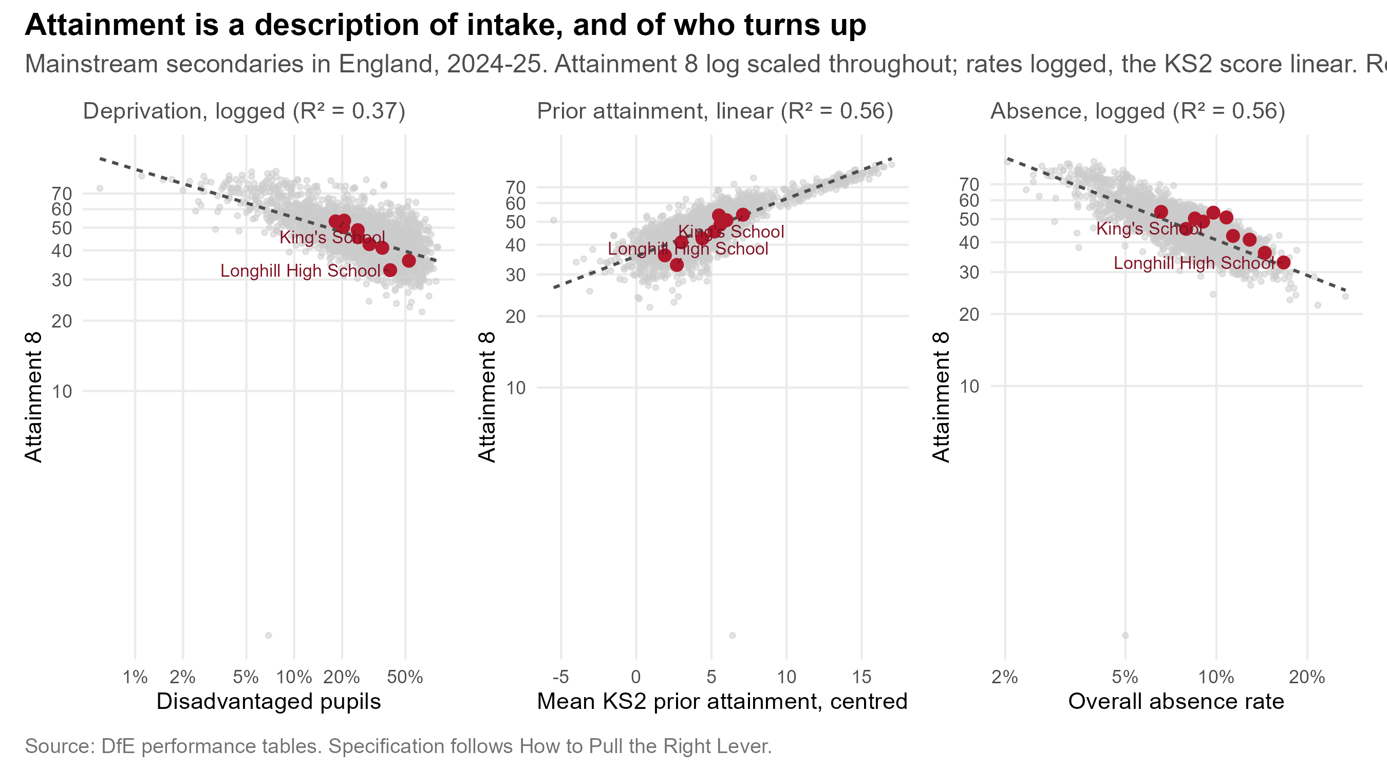
The common account is that attainment tracks deprivation. It does, but
weakly, and stopping there points the city at the wrong lever.
The specification below follows the model in
[How to Pull the Right Lever](https://adamdennett.github.io/school_attainment_tool/index.html):
Attainment 8 and the rate variables are logged, so their coefficients
are elasticities, while prior attainment enters as a mean KS2 score
because it is a score and not a rate.
Across `r fmt_n(nobs(m_fsm))` mainstream secondaries in England, the
proportion of disadvantaged pupils explains **`r fmt_pct(R2(m_fsm))`**
of the variation in Attainment 8. Prior attainment explains
**`r fmt_pct(R2(m_prior))`**. And the single strongest of the three is
neither: **absence alone explains `r fmt_pct(R2(m_abs1))`**. All three
together reach `r fmt_pct(R2(m_full))`.
The elasticities make the point more sharply than the R² values do. In
the combined model a one per cent rise in absence is associated with a
**`r sprintf("%.2f", abs(cf[["log(PERCTOT)"]]))` per cent** fall in
Attainment 8; a one per cent rise in the disadvantaged share with a fall
of just **`r sprintf("%.2f", abs(cf[["log(PTFSM6CLA1A)"]]))` per cent**
--- roughly
`r sprintf("%.0f", abs(cf[["log(PERCTOT)"]]) / abs(cf[["log(PTFSM6CLA1A)"]]))`
times smaller.
That ordering is the finding. Who is poor matters least of the three.
What children could already do at eleven matters more. Whether they are
in the room matters most.
```{r fig-att8-prior}
#| fig-cap: "Attainment 8 against two features of intake, every mainstream secondary in England in the latest year, with Brighton & Hove schools highlighted. Prior attainment and absence both order schools far more sharply than deprivation does."
#| fig-height: 5
# Attainment 8 is on a log axis in every panel, matching the model. The
# x axis is logged for the two rates and left linear for the KS2 score,
# so each panel is drawn on the scale its term is actually fitted on.
panel <- function(xvar, xlab, ttl, logx) {
d <- nat %>% filter(!is.na(.data[[xvar]]))
b <- bh_latest %>% filter(!is.na(.data[[xvar]]))
if (logx) { d <- d %>% filter(.data[[xvar]] > 0); b <- b %>% filter(.data[[xvar]] > 0) }
p <- ggplot(d, aes(.data[[xvar]], ATT8SCR)) +
geom_point(colour = "grey80", size = 0.9, alpha = 0.5) +
geom_smooth(method = "lm", formula = y ~ x, se = FALSE,
colour = "grey30", linewidth = 0.7, linetype = "22") +
geom_point(data = b, colour = "#b2182b", size = 2.4) +
ggrepel::geom_text_repel(
data = b %>% filter(SCHNAME %in% c("Longhill High School", "King's School")),
aes(label = SCHNAME), size = 2.9, colour = "#7f0f22",
min.segment.length = 0, segment.size = 0.3, seed = 1) +
scale_y_log10(breaks = c(10, 20, 30, 40, 50, 60, 70)) +
labs(x = xlab, y = "Attainment 8", subtitle = ttl) +
theme_bh(11)
if (logx)
p <- p + scale_x_log10(labels = label_percent(scale = 1),
breaks = c(1, 2, 5, 10, 20, 50))
p
}
(panel("PTFSM6CLA1A", "Disadvantaged pupils",
sprintf("Deprivation, logged (R² = %.2f)", summary(m_fsm)$r.squared), TRUE) |
panel("ks2_c", "Mean KS2 prior attainment, centred",
sprintf("Prior attainment, linear (R² = %.2f)", summary(m_prior)$r.squared), FALSE) |
panel("PERCTOT", "Overall absence rate",
sprintf("Absence, logged (R² = %.2f)", summary(m_abs1)$r.squared), TRUE)) +
plot_annotation(
title = "Attainment is a description of intake, and of who turns up",
subtitle = sprintf("Mainstream secondaries in England, %s. Attainment 8 log scaled throughout; rates logged, the KS2 score linear. Red points are Brighton & Hove.",
perf$latest),
caption = "Source: DfE performance tables. Specification follows How to Pull the Right Lever.",
theme = theme_bh())
```
Two consequences follow, and they point in the same direction.
**A headline score is mostly a description of who walks through the
door.** Once prior attainment and deprivation are accounted for,
**`r above` of the `r nrow(bh_resid)`** Brighton & Hove schools score
above what the national relationship predicts for their intake. On the
measure that isolates the school's own contribution, this is not a city
with a school quality problem.
**The lever that moves is attendance, not social mix.** Absence and
deprivation travel together, and absence is the mechanism through which
much of the deprivation effect actually operates --- which is why
redistributing disadvantaged children between schools is a far weaker
instrument than it is usually assumed to be.
::: {.callout-important appearance="simple"}
## Two cautions
**Absence is partly an outcome as well as a cause.** A child who is
disengaged attends less *and* attains less, so a single-equation fit
overstates how much of that `r fmt_pct(R2(m_full))` is absence doing the
causal work. The Lever report models this properly --- with school, year,
region and inspection-rating effects, and a first stage that models
absence itself --- rather than reading it off a scatterplot. These three
panels are an illustration of that model's premise, not a substitute for
it.
**These are single-year, single-equation fits.** The full model is
fitted on a multi-year panel with random effects and a wider set of
school characteristics, including English as an additional language,
teacher retention and admissions policy. The ordering of the three terms
here matches it; the individual R² values will not, and none of them
should be quoted as a causal effect.
:::
::: {.callout-tip}
## The detail behind this is published separately
The contextualised analysis --- value-added modelling across every local
authority in England, and what it says about where Brighton's schools
really sit --- is set out in
[How to Pull the Right Lever](https://adamdennett.github.io/school_attainment_tool/index.html).
Its central findings are that Brighton's schools perform well once
intake is accounted for, and that **absence, not social mixing, is the
largest single lever available to the city**. This document takes those
findings as given and turns to the spatial and demographic questions the
Lever report does not address.
:::
```{r fig-ranking-flip}
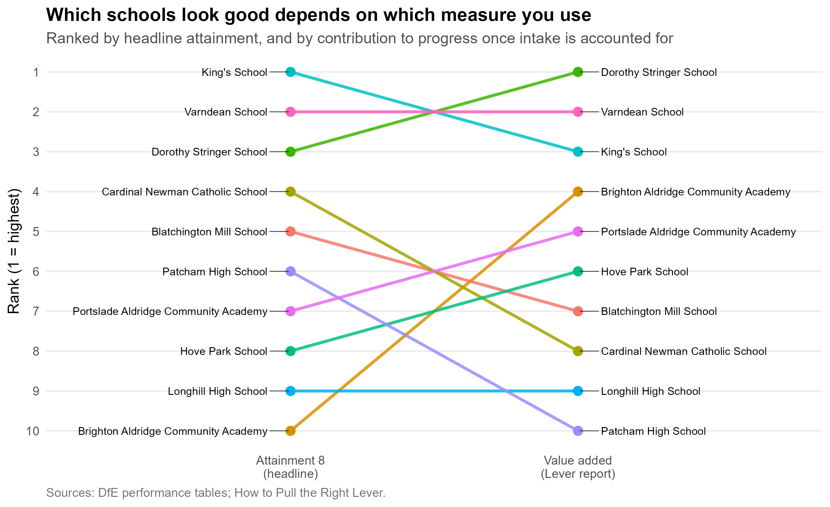
#| fig-cap: "The same ten schools ranked two ways: by headline Attainment 8, and by the value-added measure from the Lever report. Lines crossing means the two measures disagree about which schools are doing well."
#| fig-height: 5.5
flip <- oi$attract %>%
filter(!is.na(att8), !is.na(va_lever), name != "Peacehaven Community School") %>%
mutate(rank_att8 = rank(-att8), rank_va = rank(-va_lever)) %>%
select(name, rank_att8, rank_va) %>%
pivot_longer(starts_with("rank_"), names_to = "measure", values_to = "rank") %>%
mutate(measure = factor(measure, c("rank_att8", "rank_va"),
c("Attainment 8\n(headline)", "Value added\n(Lever report)")))
moved <- flip %>%
pivot_wider(names_from = measure, values_from = rank) %>%
rename(att8 = 2, va = 3) %>%
mutate(shift = att8 - va)
ggplot(flip, aes(measure, rank, group = name)) +
geom_line(aes(colour = name), linewidth = 1.1, alpha = 0.85, show.legend = FALSE) +
geom_point(aes(colour = name), size = 3, show.legend = FALSE) +
ggrepel::geom_text_repel(
data = flip %>% filter(measure == levels(flip$measure)[1]),
aes(label = name), hjust = 1, nudge_x = -0.08, size = 3,
direction = "y", segment.size = 0.2, seed = 1) +
ggrepel::geom_text_repel(
data = flip %>% filter(measure == levels(flip$measure)[2]),
aes(label = name), hjust = 0, nudge_x = 0.08, size = 3,
direction = "y", segment.size = 0.2, seed = 1) +
scale_y_reverse(breaks = 1:10) +
scale_x_discrete(expand = expansion(add = c(0.85, 0.85))) +
labs(x = NULL, y = "Rank (1 = highest)",
title = "Which schools look good depends on which measure you use",
subtitle = "Ranked by headline attainment, and by contribution to progress once intake is accounted for",
caption = "Sources: DfE performance tables; How to Pull the Right Lever.") +
theme_bh() +
theme(panel.grid.major.x = element_blank())
```
```{r flip-stats}
#| include: false
# Ties are real here - two schools fall by the same four places - so
# collapse to a list rather than letting slice_min pick one silently.
and_list <- function(x) if (length(x) < 2) x else
paste(paste(head(x, -1), collapse = ", "), "and", tail(x, 1))
up <- moved %>% filter(shift == max(shift))
down <- moved %>% filter(shift == min(shift))
n_moved3 <- sum(abs(moved$shift) >= 3)
```
The lines cross a great deal. **`r and_list(up$name)`** rises
`r abs(up$shift[1])` places when you move from the headline measure to
the value-added one; **`r and_list(down$name)`** falls
`r abs(down$shift[1])`. `r n_moved3` of the ten schools move by three
places or more.
The schools that fall are not bad schools, and the schools that rise are
not suddenly good ones. The two measures are answering different
questions: one asks what pupils at this school achieved, the other asks
how much of that the school is responsible for. Families reading the
published headline are answering the first question while believing they
are answering the second --- and section 5 shows that this has a
measurable effect on where demand actually goes.
### For disadvantaged pupils, the direction reverses {#sec-concentration-evidence}
The fall in Attainment 8 that goes with a higher disadvantaged share is
an average over all pupils. [How to Pull the Right Lever](https://adamdennett.github.io/school_attainment_tool/index.html)
fits the same model separately for disadvantaged and non-disadvantaged
pupils, and the two disagree about direction.
- **For non-disadvantaged pupils** a school with more disadvantaged
pupils is associated with lower attainment, even after their own
attendance and prior attainment are accounted for.
- **For disadvantaged pupils** it is associated with slightly *higher*
attainment, once absence and low prior attainment are accounted for.
The report finds this in the four-year panel and in each year
separately, and under different measures of disadvantaged attainment
and of school disadvantage ([robustness checks](https://adamdennett.github.io/school_attainment_tool/model_experiments.html#sec-directionality),
[model results](https://adamdennett.github.io/school_attainment_tool/model_results.html#disadvantaged-pupils)). It is strongest in the non-GCSE
qualifications of the Attainment 8 'open' element.
- **The effect is small, and it is mostly about the schools.** In the
full multilevel model the coefficient shrinks towards zero once region,
local authority and Ofsted rating are allowed for. The report's reading
is that disadvantaged pupils do not gain simply from being together;
they gain because schools with many of them --- in some places and with
some inspection records --- have learned to serve them well, including
through well-targeted vocational routes.
The report is explicit that this is **not an argument for concentrating
disadvantaged pupils**, and that mixed intakes may have benefits it does
not measure. Its argument is narrower: where a city's geography already
concentrates disadvantage in some schools, deconcentration pursued at
the cost of longer journeys is unlikely to help the pupils it is meant to
help, and may harm them.
::: {.callout-note appearance="simple"}
## Brighton Aldridge is the local example
Brighton Aldridge Community Academy has about half its pupils
disadvantaged, some of the city's highest absence, and around 30% of its
pupils arriving with low prior attainment. On the same panel model's
contextualised results, a disadvantaged pupil leaving BACA in 2024--25
did about **5.7 Attainment 8 points better** than a comparable pupil at a
similar school elsewhere in England, and about **3.1 points better on
average over four years** --- the strongest result in the city for
disadvantaged pupils, and far larger than the fraction of a point that
changing a school's disadvantage mix would be expected to deliver. Ofsted
rated the school Good in every area in April 2025.
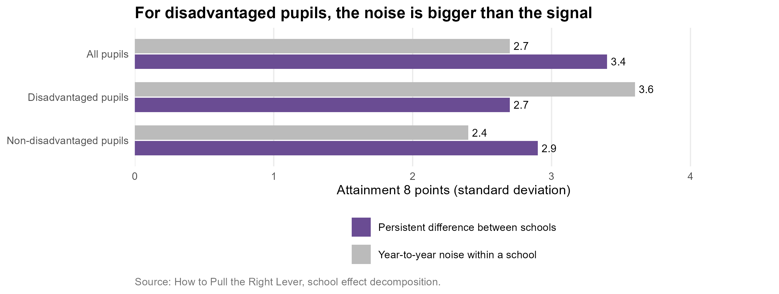
@sec-noise applies to BACA as to any school: a single year of
disadvantaged results is one draw, and the four-year figure is the one to
lean on. It is still well above anything the redistribution of pupils
could deliver.
:::
**What follows for this document.** Several options in @sec-weighing ---
Longhill at Elm Grove, Whitehawk back in Longhill's catchment --- raise
the segregation index because they put more disadvantaged children in
the same school. The council's policy aim treats that as a cost. The
national evidence does not: provided the school is organised and funded
for the intake it gets, a more concentrated intake is not a worse one for
its disadvantaged pupils. The segregation index is reported here because
the council asks for it, not because it measures harm.
## How much can a school change at all? {#sec-school-effects}
There is a prior question underneath all of this, and it is the one that
bears most directly on what the council can achieve by moving children
between schools.
```{r variance-decomp}
#| include: false
# Shapley (LMG) decomposition, following RPE_Paper.qmd. A t-value in a
# multiple regression describes each predictor's *unique* contribution,
# so where predictors are as correlated as these are it cannot rank
# them. The Shapley share instead averages each variable's incremental
# R2 across every order in which the three could enter the model, which
# is the standard way of apportioning variance that predictors share.
r2_of <- function(vs) {
rhs <- if (!length(vs)) "1" else paste(vs, collapse = " + ")
summary(lm(as.formula(paste("log(ATT8SCR) ~", rhs)), data = nat))$r.squared
}
three <- c("log(PTFSM6CLA1A)", "log(PERCTOT)", "ks2_c")
perms <- list(c(1,2,3), c(1,3,2), c(2,1,3), c(2,3,1), c(3,1,2), c(3,2,1))
shap <- setNames(numeric(3), three)
for (p in perms) {
sofar <- character(0)
for (i in p) {
v <- three[i]
shap[v] <- shap[v] + (r2_of(c(sofar, v)) - r2_of(sofar))
sofar <- c(sofar, v)
}
}
shap <- shap / length(perms)
shap_share <- 100 * shap / sum(shap)
# How much of the explained variance is shared rather than unique: the
# gap between the full model and the sum of each term's last-in
# contribution.
uniq <- vapply(three, function(v) r2_of(three) - r2_of(setdiff(three, v)),
numeric(1))
r2_all <- r2_of(three)
shared_pct <- 100 * (r2_all - sum(uniq)) / r2_all
LAB <- c("log(PTFSM6CLA1A)" = "Disadvantage",
"log(PERCTOT)" = "Absence",
"ks2_c" = "Prior attainment")
```
Since @Coleman1966, study after study has found that the share of
variation in pupils' outcomes attributable to differences *between
schools* --- as opposed to differences in the pupils they admit and the
circumstances those pupils bring with them --- is somewhere in the order
of **`r SCHOOL_LO` to `r SCHOOL_HI` per cent**. The landmark English
study settled on about a tenth [@SmithTomlinson1989], and the finding
has held up across countries and phases [@TeddlieReynolds2000].
The multilevel model behind *How to Pull the Right Lever* decomposes
that variance directly, and lands in the same place.
```{r fig-school-share}
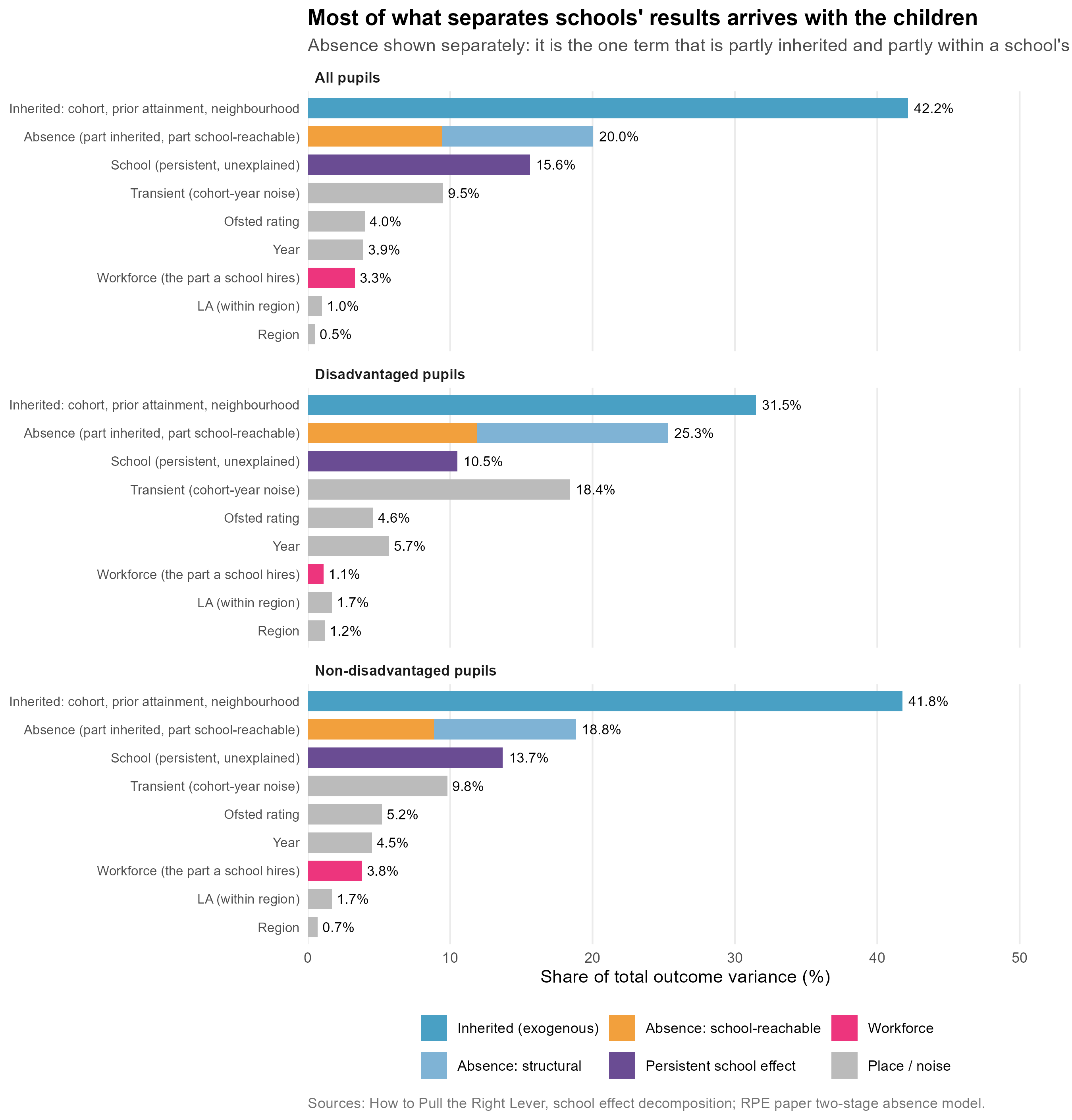
#| fig-cap: "Where the variance in school-level Attainment 8 sits, decomposed from the multilevel model, for all pupils and for the two pupil groups separately. Absence is shown as its own row rather than buried in the inherited block, split into the structural share a first-stage model predicts from intake and area, and the school-level residual it does not. The persistent school effect is an upper bound: it bundles genuine school ethos and management with anything unmeasured about the catchment, such as cultural capital or parental motivation."
#| fig-height: 9.4
sed <- bh_data("school_effect_decomp.rds")
lev <- bh_data("school_leverage.rds")
LV <- lev$leverage
GRP_COL <- c("Inherited (exogenous)" = "#49a0c4",
"Absence: structural" = "#7FB3D5",
"Absence: school-reachable" = "#F2A03D",
"Persistent school effect" = "#6A4C93",
"Workforce" = "#ED357D",
"Place / noise" = "#BBBBBB")
ABS_LAB <- "Absence (part inherited, part school-reachable)"
EXO_LAB <- "Inherited: cohort, prior attainment, neighbourhood"
# Absence is published inside the exogenous block, but it is the one
# term that is partly within a school's control. Split it out as its own
# row. The published totals are kept; the share of the exogenous block
# that is absence is taken from the fitted model, and the split of that
# absence into structural and school-reachable from the stage-1 model.
prep <- function(d, who_lab) {
r <- LV[LV$who == who_lab, ]
abs_frac <- r$absence / r$exogenous
exo_tot <- d[["Share of total %"]][grepl("^Exogenous", d$Component)]
abs_tot <- exo_tot * abs_frac
bind_rows(
d %>%
filter(!grepl("^Exogenous", Component)) %>%
transmute(Component, share = `Share of total %`,
grp_type = case_when(
grepl("^Endogenous", Component) ~ "Workforce",
Component == "School (persistent, unexplained)" ~ "Persistent school effect",
TRUE ~ "Place / noise")),
tibble(Component = EXO_LAB, share = exo_tot - abs_tot,
grp_type = "Inherited (exogenous)"),
tibble(Component = ABS_LAB,
share = c(abs_tot * lev$struct_share, abs_tot * lev$school_share),
grp_type = c("Absence: structural", "Absence: school-reachable"))
) %>%
mutate(who = who_lab,
Component = sub("^Endogenous, within-school \\(workforce\\)$",
"Workforce (the part a school hires)", Component))
}
decomp <- bind_rows(prep(sed$decomp_all, "All pupils"),
prep(sed$decomp_dis, "Disadvantaged pupils"),
prep(sed$decomp_non, "Non-disadvantaged pupils")) %>%
mutate(who = factor(who, c("All pupils", "Disadvantaged pupils",
"Non-disadvantaged pupils")),
grp_type = factor(grp_type, levels = names(GRP_COL)))
# Order rows by the all-pupil total for each component, so the three
# panels read in the same order and can be compared row by row.
ord <- decomp %>%
filter(who == "All pupils") %>%
group_by(Component) %>% summarise(t = sum(share), .groups = "drop") %>%
arrange(t) %>% pull(Component)
decomp <- decomp %>% mutate(Component = factor(Component, ord))
# One label per row, placed at the row total rather than per segment, so
# the split absence bar reads as a single quantity.
tot_lab <- decomp %>%
group_by(who, Component) %>% summarise(share = sum(share), .groups = "drop")
ggplot(decomp, aes(share, Component, fill = grp_type)) +
geom_col(width = 0.72) +
geom_text(data = tot_lab, inherit.aes = FALSE, hjust = -0.15, size = 3,
mapping = aes(x = share, y = Component,
label = sprintf("%.1f%%", share))) +
facet_wrap(~ who, ncol = 1) +
scale_fill_manual(values = GRP_COL, name = NULL) +
scale_x_continuous(limits = c(0, 52), expand = expansion(mult = c(0, 0.02))) +
guides(fill = guide_legend(nrow = 2)) +
labs(x = "Share of total outcome variance (%)", y = NULL,
title = "Most of what separates schools' results arrives with the children",
subtitle = "Absence shown separately: it is the one term that is partly inherited and partly within a school's reach",
caption = "Sources: How to Pull the Right Lever, school effect decomposition; RPE paper two-stage absence model.") +
theme_bh(11) +
theme(legend.position = "bottom", panel.grid.major.y = element_blank(),
axis.text.y = element_text(size = 8),
strip.text = element_text(face = "bold", hjust = 0))
```
```{r decomp-stats}
#| include: false
pick <- function(d, pat) d[["Share of total %"]][grepl(pat, d$Component)][1]
wf_all <- pick(sed$decomp_all, "^Endogenous")
ex_all <- pick(sed$decomp_all, "^Exogenous")
sch_all <- pick(sed$decomp_all, "^School \\(persistent")
wf_dis <- pick(sed$decomp_dis, "^Endogenous")
ex_dis <- pick(sed$decomp_dis, "^Exogenous")
sch_dis <- pick(sed$decomp_dis, "^School \\(persistent")
wf_non <- pick(sed$decomp_non, "^Endogenous")
ex_non <- pick(sed$decomp_non, "^Exogenous")
```
For all pupils, the part a school **directly controls** through the
staff it hires accounts for about **`r fmt_pct(LV$workforce[LV$who == "All pupils"], 1)`**
of the variance. What it inherits with the intake --- cohort composition,
prior attainment, neighbourhood --- accounts for roughly
**`r fmt_pct(LV$exogenous[LV$who == "All pupils"] - LV$absence[LV$who == "All pupils"], 0)`**.
Even the persistent school effect, at `r sch_all`%, is an upper bound: it
is what is left once everything measured is accounted for, so it bundles
genuine school ethos and leadership together with anything unmeasured
about the catchment --- cultural capital, parental motivation, and the
rest.
Absence has its own row because it is the one term that will not sit in
either camp. The published decomposition files it with the inherited
block, but a school's attendance is partly a fact about its intake and
partly a fact about what it does. The next section takes that apart, and
it turns out to matter more than anything else on the chart.
**For disadvantaged pupils --- the group any mixing policy is aimed at
--- the workforce term falls to `r wf_dis`%**, against `r ex_dis`%
inherited, with a persistent school effect of `r sch_dis`%. The lever
gets *smaller*, not larger, precisely where the policy is pointed. For
non-disadvantaged pupils it is `r wf_non`% against `r ex_non`% --- so
the pattern is not an artefact of one group, and the school-controllable
share is smallest for the children the policy is meant to help.
## Absence is the term that moves {#sec-absence-split}
The published decomposition files absence inside the exogenous block ---
"cohort, prior attainment, absence, neighbourhood" --- as though a school
simply receives its attendance rate. The two-stage work in the RPE paper
shows that it does not. A first-stage model of school absence on intake,
area and segregation explains only about half of its variation; the rest
is a residual that pastoral systems, attendance officers, family liaison
and persistent-absentee follow-up act on directly. That is why it is
drawn as its own split row above, and it is worth being precise about
the size of each part.
```{r leverage-stats}
#| include: false
lev <- bh_data("school_leverage.rds")
LV <- lev$leverage
lv <- function(who, col) LV[[col]][LV$who == who]
```
Across `r fmt_n(lev$stage1_n)` school-years, that first stage accounts
for **`r fmt_pct(100 * lev$struct_share)`** of the variation in absence.
The other **`r fmt_pct(100 * lev$school_share)`** is school-level
residual. Absence is not one thing: roughly half of it is structural and
outside a school's reach, and roughly half is not.
That changes the arithmetic, because absence is the largest single term
in the exogenous block --- `r fmt_pct(lv("All pupils", "absence"), 1)` of
total variance for all pupils, and
`r fmt_pct(lv("Disadvantaged pupils", "absence"), 1)` for disadvantaged
pupils, where it is the biggest component of all.
```{r fig-leverage}
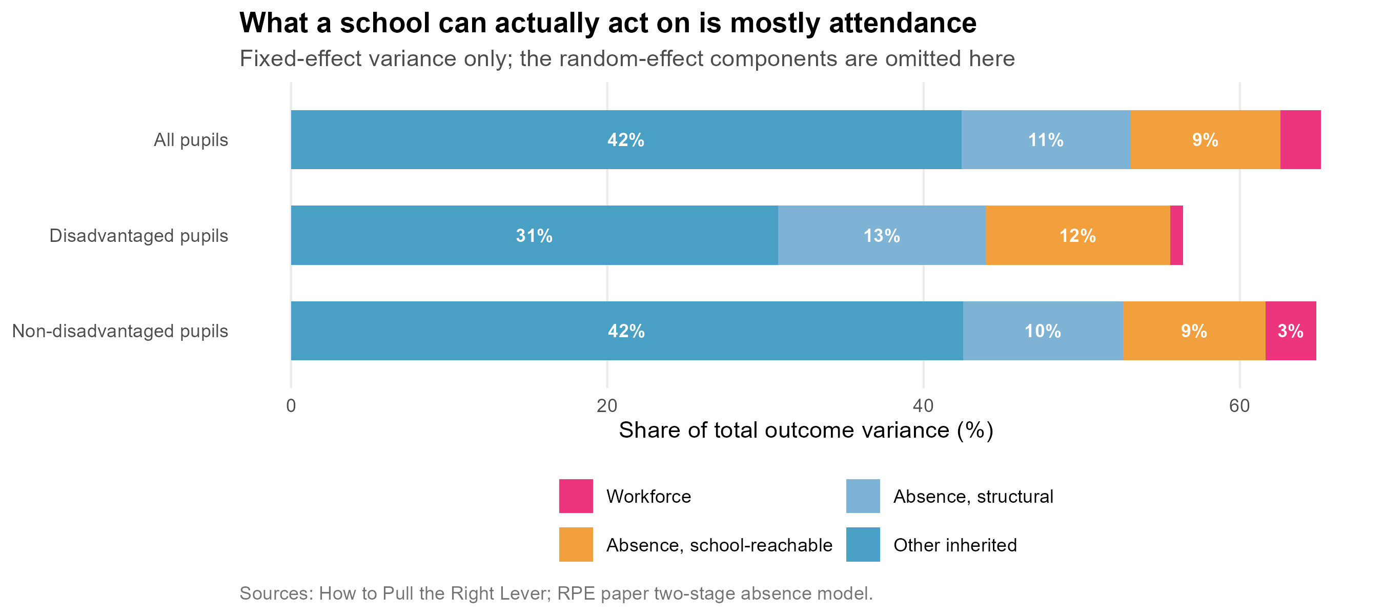
#| fig-cap: "The same variance, re-cut by what a school can actually act on. The absence term is split into the structural share the first-stage model predicts and the school-level residual it does not."
#| fig-height: 4
LV %>%
transmute(who = factor(who, LV$who),
`Workforce` = workforce,
`Absence, school-reachable` = absence_school,
`Absence, structural` = absence_structural,
`Other inherited` = exogenous - absence) %>%
pivot_longer(-who, names_to = "part", values_to = "pct") %>%
mutate(part = factor(part, c("Workforce", "Absence, school-reachable",
"Absence, structural", "Other inherited"))) %>%
ggplot(aes(pct, fct_rev(who), fill = part)) +
geom_col(width = 0.62) +
geom_text(aes(label = ifelse(pct >= 3, sprintf("%.0f%%", pct), "")),
position = position_stack(vjust = 0.5), size = 3.1,
colour = "white", fontface = "bold") +
scale_fill_manual(values = c("Workforce" = "#ED357D",
"Absence, school-reachable" = "#F2A03D",
"Absence, structural" = "#7FB3D5",
"Other inherited" = "#49a0c4"), name = NULL) +
guides(fill = guide_legend(nrow = 2)) +
labs(x = "Share of total outcome variance (%)", y = NULL,
title = "What a school can actually act on is mostly attendance",
subtitle = "Fixed-effect variance only; the random-effect components are omitted here",
caption = "Sources: How to Pull the Right Lever; RPE paper two-stage absence model.") +
theme_bh(11) +
theme(legend.position = "bottom", panel.grid.major.y = element_blank())
```
Adding the school-controllable half of absence to the workforce term
gives a school-reachable share of **`r fmt_pct(lv("All pupils", "reachable"), 1)`**
for all pupils, **`r fmt_pct(lv("Disadvantaged pupils", "reachable"), 1)`**
for disadvantaged pupils and
**`r fmt_pct(lv("Non-disadvantaged pupils", "reachable"), 1)`** for
non-disadvantaged --- strikingly consistent, and sitting squarely inside
the `r SCHOOL_LO`--`r SCHOOL_HI` per cent that sixty years of
school-effectiveness research has settled on.
::: {.callout-note appearance="simple"}
## A small discrepancy worth naming
The workforce figures in this section are recomputed from the fitted
models rather than read off the published table, so that the parts sum
to the totals quoted beside them. They come out slightly lower than the
published version --- `r fmt_pct(lv("All pupils", "workforce"), 1)`
against `r wf_all`% for all pupils --- because the cached table and the
model objects available here are not from quite the same fit. The
difference is under a percentage point and changes nothing in the
argument, but the two numbers are not identical and it would be worse to
present them as if they were.
:::
So the earlier conclusion needs restating, more precisely and more
usefully:
::: {.callout-important}
## The corrected version
A school can reach about **`r fmt_pct(lv("All pupils", "reachable"), 0)`**
of the variance in its results --- not the `r wf_all`% the workforce term
alone suggests. But **almost all of that leverage runs through
attendance**, not through who is sitting in the classroom.
For disadvantaged pupils the point is sharper still. The workforce term
is `r fmt_pct(lv("Disadvantaged pupils", "workforce"), 1)`; the
school-reachable absence term is
`r fmt_pct(lv("Disadvantaged pupils", "absence_school"), 1)` ---
`r sprintf("%.0f", lv("Disadvantaged pupils", "absence_school") / lv("Disadvantaged pupils", "workforce"))`
times larger. The lever that works for the children the policy is aimed
at is attendance, and it is not an admissions lever.
Moving children between schools does not touch either term. It changes
which building a child attends without changing their attendance, and
without changing the intake characteristics that account for the rest.
That is the case against expecting much from redistribution --- and,
equally, the case for expecting a great deal from attendance work.
:::
::: {.callout-note appearance="simple"}
## Does the shared variance change this?
It is a fair challenge. The two fixed blocks are not independent ---
schools with difficult intakes also tend to have less stable workforces
--- so the variance they share has to be allocated somehow, and the
answer depends on how.
The decomposition above credits each block with its covariance against
the total. An alternative is to split the shared part evenly, as a
Shapley decomposition does. On the fitted models the two blocks
correlate at about **+0.3 to +0.4**, and the choice is not immaterial:
the workforce share moves from 2.5% to **7.5%** for all pupils, from
0.8% to **3.1%** for disadvantaged pupils, and from 3.2% to **8.1%** for
non-disadvantaged pupils --- roughly a threefold difference.
It does not, however, change the conclusion. Under the more generous
allocation the workforce share is still about eight times smaller than
the inherited share for all pupils, and about seventeen times smaller
for disadvantaged pupils. The random-effect components --- the
persistent school effect among them --- are untouched either way,
because variance components in a multilevel model are orthogonal by
construction and have no shared part to argue over.
The figures quoted here are the published ones, on the covariance split.
Read the workforce term as *at most* a few per cent rather than as a
precise quantity.
:::
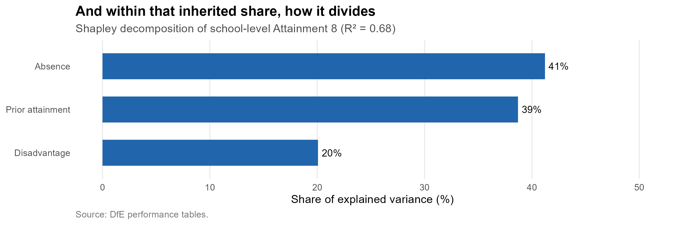
```{r fig-shapley}
#| fig-cap: "How the explained variance in school-level Attainment 8 divides between the three main intake measures, by Shapley decomposition."
#| fig-height: 3
tibble(term = LAB[three], share = shap_share) %>%
ggplot(aes(reorder(term, share), share)) +
geom_col(fill = "#2166ac", width = 0.6) +
geom_text(aes(label = fmt_pct(share, 0)), hjust = -0.18, size = 3.4) +
coord_flip() +
scale_y_continuous(limits = c(0, max(shap_share) * 1.22)) +
labs(x = NULL, y = "Share of explained variance (%)",
title = "And within that inherited share, how it divides",
subtitle = sprintf("Shapley decomposition of school-level Attainment 8 (R² = %.2f)", r2_all),
caption = "Source: DfE performance tables.") +
theme_bh(11) +
theme(panel.grid.major.y = element_blank())
```
Two things follow, and together they are the most important finding in
this section for the decisions in front of the council.
**Moving children between schools operates on the small term.**
Redistributing pupils changes *which* school a child attends. It does
not change the intake characteristics and social circumstances that
account for `r ex_all`% of the variance, and it does not touch the
workforce that accounts for `r wf_all`%. A policy of social mixing
through admissions is therefore working on the smaller term by
construction --- not because mixing is undesirable, but because the
arithmetic limits what it can deliver.
The next section qualifies this in an important way. One large item
inside that `r ex_all`% is not inherited at all.
**And the measured drivers cannot be cleanly separated anyway.** Of the
`r fmt_pct(100 * r2_all, 0)` of school-level variation the three
measures jointly explain, **`r fmt_pct(shared_pct, 0)` is variance they
*share*** rather than variance any one of them owns. Disadvantage,
absence and prior attainment correlate at
`r sprintf("%.2f", cor(log(nat$PTFSM6CLA1A), nat$ks2_c))`,
`r sprintf("%.2f", cor(log(nat$PERCTOT), nat$ks2_c))` and
`r sprintf("%.2f", cor(log(nat$PTFSM6CLA1A), log(nat$PERCTOT)))`
because they are substantially the same phenomenon seen three ways. Any
policy that targets one of them in isolation --- and an admissions
policy targets disadvantage in isolation --- is pulling on a rope
attached to the other two.
::: {.callout-important}
## What this does and does not say
It does **not** say schools do not matter. A persistent school effect of
`r sch_all`% across three and a half thousand secondary schools is a
great deal, and section 2.3 showed Brighton's schools mostly performing
above what their intakes predict. Nor does it say that segregation
between schools is acceptable; there are fairness arguments for mixed
intakes that have nothing to do with attainment.
What it says is narrower and harder to argue with: **the council should
not expect a redistribution policy to move attainment much**, because
the mechanism it operates through is the smallest of the terms
available. The instruments that reach the larger terms --- attendance
above all --- are not admissions instruments at all.
:::
## A school's disadvantaged results are a noisy signal {#sec-noise}
One row on that chart is easy to skip past and should not be. For
disadvantaged pupils, **transient cohort-year noise is the
second-largest component of all** --- larger than the persistent school
effect, larger than absence, larger than anything except what the
children bring with them.
```{r noise-stats}
#| include: false
pt <- function(d, pat) d[["Att8 points"]][grepl(pat, d$Component)][1]
sc <- function(d, pat) d[["Share of total %"]][grepl(pat, d$Component)][1]
noise <- tibble(
who = factor(c("All pupils", "Disadvantaged pupils", "Non-disadvantaged pupils"),
c("All pupils", "Disadvantaged pupils", "Non-disadvantaged pupils")),
persistent = c(pt(sed$decomp_all, "^School \\(persistent"),
pt(sed$decomp_dis, "^School \\(persistent"),
pt(sed$decomp_non, "^School \\(persistent")),
transient = c(pt(sed$decomp_all, "^Transient"),
pt(sed$decomp_dis, "^Transient"),
pt(sed$decomp_non, "^Transient")))
n_dis_tr <- pt(sed$decomp_dis, "^Transient")
n_dis_sch <- pt(sed$decomp_dis, "^School \\(persistent")
n_all_tr <- pt(sed$decomp_all, "^Transient")
n_all_sch <- pt(sed$decomp_all, "^School \\(persistent")
# Two schools with identical true performance still differ by this much
# in a given year, on average, purely from cohort-year variation.
gap_dis <- n_dis_tr * sqrt(2)
```
```{r fig-noise}
#| fig-cap: "The persistent difference between schools against the year-to-year wobble within them, in Attainment 8 points. For disadvantaged pupils the wobble is the larger of the two."
#| fig-height: 3.4
noise %>%
pivot_longer(-who, names_to = "part", values_to = "pts") %>%
mutate(part = factor(part, c("persistent", "transient"),
c("Persistent difference between schools",
"Year-to-year noise within a school"))) %>%
ggplot(aes(pts, fct_rev(who), fill = part)) +
geom_col(position = position_dodge(width = 0.72), width = 0.66) +
geom_text(aes(label = sprintf("%.1f", pts)),
position = position_dodge(width = 0.72), hjust = -0.25, size = 3.2) +
scale_fill_manual(values = c("Persistent difference between schools" = "#6A4C93",
"Year-to-year noise within a school" = "#BBBBBB"),
name = NULL) +
scale_x_continuous(limits = c(0, max(noise$transient) * 1.25),
expand = expansion(mult = c(0, 0.02))) +
guides(fill = guide_legend(nrow = 2)) +
labs(x = "Attainment 8 points (standard deviation)", y = NULL,
title = "For disadvantaged pupils, the noise is bigger than the signal",
caption = "Source: How to Pull the Right Lever, school effect decomposition.") +
theme_bh(11) +
theme(legend.position = "bottom", panel.grid.major.y = element_blank())
```
For **all** pupils the school signal wins: the persistent difference
between schools is `r sprintf("%.1f", n_all_sch)` Attainment 8 points
against `r sprintf("%.1f", n_all_tr)` points of year-to-year noise. For
**disadvantaged** pupils it reverses --- `r sprintf("%.1f", n_dis_sch)`
points of persistent difference against **`r sprintf("%.1f", n_dis_tr)`
points of noise**.
The reason is arithmetic rather than mysterious. A secondary school's
disadvantaged cohort is small --- often forty or fifty pupils --- and
small numbers move about. A handful of children having a bad year, or a
good one, shifts the published figure by more than any real difference
in what the school does.
The consequence is uncomfortable and worth stating plainly. **Two
schools doing genuinely equally well by their disadvantaged pupils will
differ by around `r sprintf("%.0f", gap_dis)` Attainment 8 points in a
given year for no reason at all.** That is larger than most of the gaps
that get argued about. A single year of disadvantaged results is not
evidence about a school; it is one draw from a distribution.
::: {.callout-important}
## What follows for how the city reads its own data
**Never judge a school on one year of disadvantaged results.** Three or
more years, averaged, or the comparison is mostly noise. This applies to
league tables, to consultation documents, and to the case made for or
against any individual school.
**Do not expect to detect an admissions policy's effect this way
either.** If redistribution moves disadvantaged attainment by a point or
two --- which section 2.4 suggests is optimistic --- that signal sits
well inside `r sprintf("%.0f", gap_dis)` points of year-to-year variation.
The policy could work exactly as intended and be invisible for years;
it could also fail and appear to succeed. Evaluating it will need
attendance and intake measures, not headline outcomes.
**This bears directly on the free school meals review.** The FSM
admissions priority took effect for entry in September 2023. Those
children entered Year 7 that autumn and will not sit GCSEs until
**summer 2028**. So a review conducted now is not working with thin
outcome evidence --- it is working with *none*: not one cohort admitted
under the policy has yet reached an examination. Even in 2028 there will
be a single cohort, and a single cohort of disadvantaged pupils in one
catchment carries the `r sprintf("%.1f", n_dis_tr)`-point year-to-year
variation described above.
That is not an argument against reviewing the policy. Admission
patterns, intake composition by catchment, and the operation of the
criteria itself can all be examined now, and section 5 does some of
that. It is an argument against reviewing it **on attainment**, or
against any conclusion of the form "results have or have not improved
since the policy came in". No honest analysis can support such a claim
from the data that exists, in either direction.
**This compounds the problem in section 2.3.** Families are choosing on
a measure that is largely a description of intake, *and* that measure is
noisiest precisely for the pupils whose schools are most often
criticised on it.
:::
# Demographic futures {#sec-demography}
The single most important fact about this system is that it is shrinking,
and that the shrinkage is already locked in. The children who will enter
Year 7 in 2033 have already started primary school. Their number is not
a forecast in any meaningful sense --- it is a count, adjusted for a
transfer rate that has been remarkably stable for a decade.
## What has already happened {#sec-cohort-history}
```{r cohort-data}
#| include: false
rc <- bh_data("reception_cohort.rds")
y7 <- rc$secondary_city
rec <- rc$reception_city
peak <- y7 %>% slice_max(y7_offers, n = 1)
now <- y7 %>% slice_max(year, n = 1)
proj <- rc$projection
last_proj <- proj %>% slice_max(entry_year, n = 1)
drop_pct <- 100 * (last_proj$central - now$y7_offers) / now$y7_offers
```
Year 7 offers across the city peaked at **`r fmt_n(peak$y7_offers)`** in
`r peak$year`. In `r now$year` the figure was
**`r fmt_n(now$y7_offers)`** --- a fall of
`r fmt_pct(100 * (peak$y7_offers - now$y7_offers) / peak$y7_offers, 1)`
from the peak. That decline is not a projection. It has happened.
```{r fig-cohort-history}
#| fig-cap: "Reception and Year 7 offers made across Brighton & Hove. The reception line leads the Year 7 line by seven years, so it is a preview of secondary demand rather than a separate story."
#| fig-height: 5
bind_rows(
y7 %>% transmute(year, offers = y7_offers, phase = "Year 7 offers"),
rec %>% transmute(year, offers = rec_offers, phase = "Reception offers")) %>%
ggplot(aes(year, offers, colour = phase)) +
geom_line(linewidth = 1.1) +
geom_point(size = 2) +
scale_colour_manual(values = c("Reception offers" = "#2c7fb8",
"Year 7 offers" = "#b2182b"), name = NULL) +
scale_y_continuous(labels = label_comma(), limits = c(0, NA)) +
labs(x = NULL, y = "Offers made",
title = "Both phases are past their peak",
subtitle = "Reception offers turn down first, and Year 7 follows seven years later",
caption = "Source: BHCC published allocation factsheets.") +
theme_bh()
```
## The cohort already in school {#sec-projection}
The transfer rate from a reception cohort to the Year 7 cohort seven
years later has been strikingly stable. Across the six cohorts where
both ends are observable, **`r fmt_pct(100 * rc$survival_recent, 1)`** of
reception offers reappear as Year 7 offers, with a standard deviation of
just `r fmt_pct(100 * rc$survival_sd, 1)`. The city loses about one child
in nine between ages four and eleven --- to independent schools, to
moves out of the area, and to schools across the boundary.
Applying that rate to reception cohorts already in school gives a
projection that depends on almost no assumptions:
```{r fig-projection}
#| fig-cap: "Year 7 demand projected from reception cohorts already in school. The band is the range implied by the observed year-to-year variation in the transfer rate."
#| fig-height: 5
ggplot() +
geom_ribbon(data = proj, aes(entry_year, ymin = lo, ymax = hi),
fill = "#b2182b", alpha = 0.18) +
geom_line(data = proj, aes(entry_year, central),
colour = "#b2182b", linewidth = 1.1, linetype = "22") +
geom_point(data = proj, aes(entry_year, central), colour = "#b2182b", size = 2) +
geom_line(data = y7, aes(year, y7_offers), colour = "grey25", linewidth = 1.1) +
geom_point(data = y7, aes(year, y7_offers), colour = "grey25", size = 2) +
annotate("text", x = 2016, y = 2480, label = "Observed", colour = "grey25",
hjust = 0, fontface = "bold", size = 3.6) +
annotate("text", x = 2029.5, y = 2180, label = "Projected from\nchildren already in school",
colour = "#b2182b", hjust = 0, size = 3.4, lineheight = 0.95) +
scale_y_continuous(labels = label_comma(), limits = c(0, NA)) +
labs(x = NULL, y = "Year 7 offers",
title = sprintf("A further %s fall is already in the primary schools",
fmt_pct(abs(drop_pct), 0)),
subtitle = sprintf("From %s in %s to about %s by %s",
fmt_n(now$y7_offers), now$year,
fmt_n(last_proj$central), last_proj$entry_year),
caption = "Sources: BHCC allocation factsheets; transfer rate estimated from six observed cohorts.") +
theme_bh()
```
By **`r last_proj$entry_year`** the city should expect about
**`r fmt_n(last_proj$central)`** Year 7 children, against
`r fmt_n(now$y7_offers)` today --- a further fall of
`r fmt_pct(abs(drop_pct), 0)`. Against a current published admission
capacity of about
`r fmt_n(sum(oi$schools$pan2026[oi$schools$name != "Peacehaven Community School"]))`
places, that is roughly
`r fmt_n(sum(oi$schools$pan2026[oi$schools$name != "Peacehaven Community School"]) - last_proj$central)`
surplus places --- the equivalent of two and a half average-sized
secondary schools standing empty.
## Where the council's forecast differs {#sec-council-forecast}
The council publishes its own catchment-level forecasts. They are
consistently **higher** than what the primary cohorts support, and the
gap widens with distance.
```{r fig-forecast-gap}
#| fig-cap: "The council's own demand forecast against a projection built from reception cohorts already in school. Positive values mean the council expects more children than the primary registers contain."
#| fig-height: 4.6
rc$comparison %>%
mutate(gap = ons_demand - reception_based) %>%
ggplot(aes(entry_year, gap)) +
geom_col(fill = "#7b3294", alpha = 0.85, width = 0.65) +
geom_hline(yintercept = 0, colour = "grey30") +
geom_text(aes(label = sprintf("%+.0f", gap),
vjust = ifelse(gap >= 0, -0.4, 1.3)), size = 3.2) +
scale_y_continuous(expand = expansion(mult = c(0.15, 0.18))) +
labs(x = "Year of Year 7 entry", y = "Council forecast minus cohort projection",
title = "The council expects more children than the primary registers hold",
subtitle = "Difference in Year 7 places, city-wide",
caption = "Sources: BHCC published forecasts; reception-based projection as above.") +
theme_bh()
```
The city-wide figure hides a good deal. Broken down by catchment, and
set against the council's own two successive forecasts, the picture is
less tidy.
```{r fig-catchment-projections}
#| fig-cap: "Year 7 offers for each catchment: what has actually happened, our projection from primary cohorts already in school, and the council's two most recent forecasts of the same years. Dotted line is the catchment's admission number."
#| fig-height: 8
#| fig-width: 10
# Four series on one set of axes. The council labels its catchments
# differently from the model tables, so everything is converted to model
# keys first - see as_model_catchment() in R/00_core.R.
CATCH_DISPLAY <- c(CATCH_LABELS[unname(CATCH_FROM_MODEL)], "Religious schools")
names(CATCH_DISPLAY) <- c(names(CATCH_FROM_MODEL), "Religious schools")
council25 <- rc$council %>%
transmute(catchment = as_model_catchment(CatchmentGroup),
entry_year, offers = council, PAN,
series = "Council forecast (Oct-25)")
council24 <- bh_data("council_forecast_oct24.csv") %>%
transmute(catchment = as_model_catchment(CatchmentGroup),
entry_year, offers = council_oct24,
series = "Council forecast (Oct-24, superseded)")
series <- bind_rows(
rc$observed_by_catchment %>%
transmute(catchment, entry_year, offers = y7_offers,
series = "Actual offers"),
rc$by_catchment %>%
transmute(catchment, entry_year, offers = projected,
series = "Our projection (from primary cohorts)"),
council25 %>% select(-PAN),
council24) %>%
filter(!is.na(catchment), entry_year >= 2016) %>%
mutate(panel = factor(unname(CATCH_DISPLAY[catchment]),
unname(CATCH_DISPLAY)),
series = factor(series, c(
"Actual offers", "Our projection (from primary cohorts)",
"Council forecast (Oct-25)",
"Council forecast (Oct-24, superseded)")))
stopifnot(!any(is.na(series$panel)))
pan_lines <- council25 %>%
distinct(catchment, PAN) %>%
mutate(panel = factor(unname(CATCH_DISPLAY[catchment]), unname(CATCH_DISPLAY)))
ggplot(series, aes(entry_year, offers, colour = series)) +
geom_hline(data = pan_lines, aes(yintercept = PAN),
linetype = "dotted", colour = "grey30", linewidth = 0.45) +
geom_line(linewidth = 0.75) +
geom_point(size = 1.2) +
facet_wrap(~ panel, ncol = 2, scales = "free_y") +
scale_colour_manual(values = c(
"Actual offers" = "#1f78b4",
"Our projection (from primary cohorts)" = "#33a02c",
"Council forecast (Oct-25)" = "#e31a1c",
"Council forecast (Oct-24, superseded)" = "#fb9a99"), name = NULL) +
scale_y_continuous(limits = c(0, NA)) +
guides(colour = guide_legend(nrow = 2)) +
labs(x = NULL, y = "Year 7 offers",
title = "Every catchment, four views of the same future",
subtitle = "Dotted line is the catchment admission number",
caption = "Sources: BHCC allocation factsheets; BHCC forecasts, Appendices 6 and 7.") +
theme_bh(11) +
theme(legend.position = "top", strip.text = element_text(face = "bold"),
axis.text.x = element_text(angle = 45, hjust = 1))
```
```{r proj-stats}
#| include: false
# How far the council moved between its own two forecasts, on the years
# both cover - a measure of how settled the council's own view is.
rev <- inner_join(
council25 %>% select(catchment, entry_year, oct25 = offers),
council24 %>% select(catchment, entry_year, oct24 = offers),
by = c("catchment", "entry_year")) %>%
mutate(shift = oct25 - oct24)
rev_by_catch <- rev %>%
group_by(catchment) %>%
summarise(mean_shift = mean(shift), max_abs = max(abs(shift)), .groups = "drop") %>%
arrange(desc(abs(mean_shift)))
biggest_rev <- rev_by_catch %>% slice(1)
n_down <- sum(rev_by_catch$mean_shift < 0)
n_catch <- nrow(rev_by_catch)
# Where our projection sits relative to the council's current forecast,
# on the years both cover.
gap_by_catch <- inner_join(
council25 %>% select(catchment, entry_year, council = offers),
rc$by_catchment %>% select(catchment, entry_year, ours = projected),
by = c("catchment", "entry_year")) %>%
group_by(catchment) %>%
summarise(mean_gap = mean(ours - council), .groups = "drop") %>%
arrange(mean_gap)
n_below <- sum(gap_by_catch$mean_gap < 0)
closest <- gap_by_catch %>% slice_min(abs(mean_gap), n = 1)
closest_txt <- if (abs(closest$mean_gap) < 1) "under a place" else
sprintf("%.0f places", abs(closest$mean_gap))
spell <- function(n) c("one","two","three","four","five","six","seven",
"eight","nine","ten")[n]
down_txt <- if (n_down == n_catch)
sprintf("Every one of the %s catchments was", spell(n_catch)) else
sprintf("%s of the %s catchments were", spell(n_down), spell(n_catch))
```
Two things stand out.
**Our projection sits below the council's in
`r n_below` of the `r nrow(gap_by_catch)` catchments** --- the city-wide
gap of the previous chart, distributed. The closest agreement is in
`r CATCH_DISPLAY[[as.character(closest$catchment)]]`, where the two
differ by `r closest_txt` a year on average.
**And the council's own view has moved a long way in a single year.**
Between the Oct-24 and Oct-25 forecasts, for the years both cover, the
figure for
**`r CATCH_DISPLAY[[as.character(biggest_rev$catchment)]]`** moved by an
average of `r sprintf("%+.0f", biggest_rev$mean_shift)` places a year,
with a largest single-year revision of `r biggest_rev$max_abs`.
The direction is the part worth noting. **`r down_txt` revised downward**, none upward. That is not
forecasting noise; it is a consistent correction in one direction, and
it points the same way as the projection from primary cohorts. The
council's own figures are moving toward the lower number --- they have
not arrived at it yet, and decisions with twenty-year consequences are
being taken against a quantity still in motion.
## The forecast is not wrong in total. It is wrong by place {#sec-forecast-errors}
The comparison above sets one projection against another, and a reader
is entitled to ask why either should be believed. For 2026 that question
can be settled, because the offers have been made. Both the council's
forecast and our projection can be checked against what happened.
```{r tbl-2026-errors}
#| tbl-cap: "Year 7 offers in 2026: what the council forecast, what our projection gave, and what actually happened."
err26 <- rc$observed_by_catchment %>%
filter(entry_year == 2026) %>%
select(catchment, actual = y7_offers) %>%
inner_join(council25 %>% filter(entry_year == 2026) %>%
select(catchment, PAN, council = offers), by = "catchment") %>%
left_join(rc$by_catchment %>% filter(entry_year == 2026) %>%
select(catchment, ours = projected), by = "catchment") %>%
mutate(council_err = council - actual, ours_err = round(ours - actual)) %>%
arrange(desc(council_err))
err26 %>%
transmute(Catchment = unname(CATCH_DISPLAY[catchment]),
PAN, Actual = actual,
`Council forecast` = council,
`Council error` = sprintf("%+d", council_err),
`Our projection` = round(ours),
`Our error` = sprintf("%+d", ours_err)) %>%
knitr::kable(align = "lrrrrrr")
```
```{r err-stats}
#| include: false
net_err <- sum(err26$council_err)
abs_err <- sum(abs(err26$council_err))
lh26 <- err26 %>% filter(catchment == "Longhill")
hb26 <- err26 %>% filter(catchment == "Hove_Blatch")
paca26 <- err26 %>% filter(catchment == "PACA")
lh_ratio <- lh26$council / lh26$actual
```
::: {.callout-note appearance="simple"}
## Read our column with more suspicion than the council's
The council's forecast is a genuine prediction: published in advance,
checked here against what happened. Ours is not, quite. The retention
ratio it uses is fitted on cohorts that include the 2019 reception
group, which *is* the 2026 Year 7 group --- so 2026 is partly inside the
window our method was calibrated on, and its apparent accuracy is
flattered. The honest comparison is between the council's forecast and
the outturn; our column is there for orientation, not as a claim to have
done better.
:::
City-wide the council's 2026 forecast was close: it was
`r sprintf("%+d", net_err)` places out in total, on a cohort of over two
thousand. By catchment it was not close at all. The individual errors
sum to `r abs_err` places in absolute terms --- roughly
`r sprintf("%.0f", abs_err / abs(net_err))` times the net error. The
council is forecasting the right number of children and putting a great
many of them in the wrong place.
Two catchments carry most of that, and they miss in opposite directions.
**Longhill was forecast `r lh26$council` and received `r lh26$actual`
--- `r sprintf("%.1f", lh_ratio)` times too high.** This is a catchment
whose admission number is `r lh26$PAN` and which filled
`r fmt_pct(100 * lh26$actual / lh26$PAN, 0)` of it. The council's own
method already applies the largest leakage deduction in the city to this
catchment, at over 22 per cent, and it is still not close.
**Hove Park / Blatchington Mill was forecast `r hb26$council` and
received `r hb26$actual`** --- `r abs(hb26$council_err)` places too low,
the largest under-estimate of any catchment.
::: {.callout-warning}
## Question for the council 1: why is the forecast wrong in these two places, and in opposite directions?
The Hove Park / Blatchington Mill under-estimate has a candidate
explanation. The neighbouring PACA catchment was over-forecast by
`r paca26$council_err` places --- close to the
`r abs(hb26$council_err)` that Hove Park / Blatchington Mill was under
by. Children the model expected to appear in Portslade appearing in Hove
instead would account for much of it. That is testable, and the council
holds the data to test it.
**Longhill has no such explanation.** Its neighbours were not
over-forecast in a way that could absorb an
`r sprintf("%+d", lh26$council_err)`-place error --- BACA was
`r sprintf("%+d", err26$council_err[err26$catchment == "BACA"])` and
Patcham `r sprintf("%+d", err26$council_err[err26$catchment == "Patcham"])`.
The children the council expected to enrol at Longhill did not turn up
in an adjacent catchment. They did not turn up at all.
So the questions are:
1. **What accounts for the Longhill over-forecast, if not
cross-catchment movement?** Out-of-city flow to Lewes district and
the independent sector are the obvious candidates, and the council
holds allocation records that would separate them.
2. **Is the leakage rate for the Longhill catchment being estimated on
data old enough to predate the change it is meant to capture?** A
rate calibrated on historical patterns will lag a shift that is
still happening.
3. **Is the Hove Park / Blatchington Mill under-estimate the
counterpart of the PACA over-estimate?** If so, the model's
catchment-of-residence assumption is diverging from where families
actually apply, and the two errors should be corrected together
rather than separately.
These matter because the Longhill decision is being taken against the
forecast, and the forecast has been wrong about Longhill by a factor of
`r sprintf("%.1f", lh_ratio)` in the most recent year it can be checked
against.
:::
```{r lh-gap}
#| include: false
lh_council <- rc$council %>%
mutate(catchment = as_model_catchment(CatchmentGroup)) %>%
filter(catchment == "Longhill")
lh_cohort <- rc$by_catchment %>% filter(catchment == "Longhill")
lh_join <- lh_council %>%
inner_join(lh_cohort %>% select(entry_year, projected), by = "entry_year") %>%
mutate(gap = council - projected)
stopifnot(nrow(lh_join) > 0)
```
The city-wide gap is modest in most years. Broken down by catchment it
is not, and Longhill is where it opens widest.
```{r fig-longhill-gap}
#| fig-cap: "Longhill catchment: the council's forecast, the projection from its own primary cohorts, and the school's admission number."
#| fig-height: 4.6
lh_join %>%
select(entry_year, Council = council, `From primary cohorts` = projected) %>%
pivot_longer(-entry_year, names_to = "series", values_to = "children") %>%
ggplot(aes(entry_year, children, colour = series)) +
geom_hline(yintercept = rc$council_lh_pan, linetype = "31", colour = "grey45") +
annotate("text", x = min(lh_join$entry_year), y = rc$council_lh_pan + 7,
label = sprintf("Admission number (%s)", rc$council_lh_pan),
hjust = 0, size = 3.1, colour = "grey35") +
geom_line(linewidth = 1.1) + geom_point(size = 2.4) +
scale_colour_manual(values = c("Council" = "#7b3294",
"From primary cohorts" = "#008837"), name = NULL) +
scale_y_continuous(limits = c(0, NA)) +
labs(x = "Year of Year 7 entry", y = "Children",
title = "Longhill: the two forecasts disagree, and both sit below the admission number",
subtitle = sprintf("Mean gap of %.0f children a year",
mean(lh_join$gap, na.rm = TRUE)),
caption = "Sources: BHCC catchment forecasts; reception-based projection.") +
theme_bh()
```
The council's forecast for the Longhill catchment runs an average of
**`r fmt_n(mean(lh_join$gap, na.rm = TRUE))` children a year above** what
that catchment's own primary cohorts support. Both series sit below the
school's admission number of `r rc$council_lh_pan` in every year. This
matters because decisions about Longhill's future are being taken
against the higher of two numbers, and the higher one is the one the
primary registers do not support.
## The Peacehaven accession {#sec-peacehaven}
```{r peacehaven}
#| include: false
area_children <- oi$zones %>%
group_by(area) %>%
summarise(lsoas = n_distinct(lsoa), children = sum(Oi, na.rm = TRUE),
.groups = "drop")
exp_area <- area_children %>% filter(area == "Expansion area")
tot_children <- sum(area_children$children)
ph_pan <- oi$schools$pan2026[oi$schools$name == "Peacehaven Community School"]
```
The catchment system reaches beyond the city boundary. The Peacehaven
and Telscombe area contributes **`r exp_area$lsoas` LSOAs** and about
**`r fmt_n(exp_area$children)` cohort-aged children**, roughly
`r fmt_pct(100 * exp_area$children / tot_children, 0)`
of the total the model covers.
In headcount terms this is close to self-supporting: Peacehaven
Community School has an admission number of `r ph_pan`, against about
`r fmt_n(exp_area$children)` children in its area. The difficulty is not
the arithmetic but the direction of travel. These families sit at the
eastern end of a transport network that runs east--west along the coast,
and section 4 shows that they are among the least well served in the
whole study area --- not because they are far from *a* school, but
because they are far from *most* schools, and therefore have the fewest
alternatives if their first choice is full.
# How reachable are the schools? {#sec-access}
Almost all of the public argument about Brighton's schools is conducted
in terms of admissions rules --- catchments, priorities, tie-breaks.
Underneath the rules sits a physical constraint that no rule can undo:
how long it actually takes a eleven-year-old to get to each school on a
bus. This section establishes that constraint before section 5 returns
to the rules.
All journey times here are routed with `r5r` over the merged street
network and bus timetable for the area, for a weekday morning arrival.
They include walking to the stop, waiting, the ride itself, and any
transfer.
## What counts as a long journey to school? {#sec-benchmarks}
Before mapping anything it is worth fixing what these minutes mean,
because a number like "twenty-eight minutes" is only interpretable
against something.
```{r benchmark-stats}
#| include: false
bm <- acc$benchmarks
sta <- acc$statutory
```
| Benchmark | Figure | Source |
|:--|:--|:--|
| Average one-way school trip, England | **`r bm$nts_min` minutes** | National Travel Survey, five-year average to 2019 |
| Average one-way trip distance | **`r bm$nts_miles` miles** | as above |
| Statutory maximum, secondary age | **`r bm$dfe_max_sec` minutes** each way | DfE home-to-school travel guidance |
| Statutory maximum, primary age | **`r bm$dfe_max_pri` minutes** each way | as above |
Two cautions about the `r bm$nts_min`-minute average. It covers **ages 5
to 16 together**, and secondary journeys are longer than primary ones,
so it understates the secondary figure. And it counts **all modes**,
including the car --- which carries
`r 30`% of secondary school trips nationally against
`r 18`% by local bus. The journeys modelled here are walking and bus
only, so they describe the trip facing a family without a car. That is
the right comparison for this document, but it is not a like-for-like
one with the national number.
The `r bm$dfe_max_sec`-minute figure is firmer. It is the Department for
Education's guidance on how long a home-to-school journey should
reasonably take for a child of secondary age, each way, including
walking to a pick-up point.
::: {.callout-important}
## A correction to the routed times, and why it matters
The routed matrix returns a walk-and-bus itinerary for every
neighbourhood-school pair. Where the bus network is awkward it returns a
poor one: **`r fmt_pct(100 * acc$walk_fallback$share, 0)` of the
`r fmt_n(acc$walk_fallback$total)` neighbourhood-school pairs were
modelled as taking longer than simply walking the distance would**. In
the worst case a journey of about four kilometres came out at 99
minutes.
That is a property of the router, not of the city. A family facing a
99-minute bus ride to a school four kilometres away walks instead. So
every journey is now the **lesser of the routed bus time and the time it
would take to walk**, and the bus is used only where it is genuinely
faster.
The walking pace is not invented. Kent et al. [-@Kent2026], a systematic
review of active school travel, finds children's mean walking trip to
school is **`r fmt_n(acc$walk_fallback$review$dist_m)` metres in
`r sprintf("%.1f", acc$walk_fallback$review$time_min)` minutes** ---
`r sprintf("%.2f", acc$walk_fallback$kmh)` km/h --- and that is the speed
used, with a circuity factor of `r acc$walk_fallback$circuity` to turn
straight-line distance into street distance.
::: {.callout-note appearance="simple"}
## This is a ceiling, not a claim about how children travel
The same review finds children walk about a kilometre on average and
seldom beyond `r fmt_n(acc$walk_fallback$review$dist_range[2])` metres.
Capping a four-kilometre journey at its walking time does **not** assert
that a child walks four kilometres. It asserts that no journey should be
*modelled* as costing more than walking would, because a family with
that option would take it. The cap is an upper bound on modelled cost,
not a mode assumption.
:::
The correction is not cosmetic, and it is applied **upstream, in the
open model's own inputs** --- so every section of this document and of
the technical companion now uses the corrected costs. Sections 7 and 8
were re-run against them. It is worth being open that an earlier version
of this analysis overstated the headline figures:
| | Uncorrected | With the walk fallback |
|:--|--:|--:|
| Journey to the nearest school, child-weighted | 22.8 min | **`r sprintf("%.1f", acc$city$near_now)` min** |
| Neighbourhoods reaching no place within 30 min | 37 | **`r acc$city$zero30_now`** |
| Children in those neighbourhoods | 474 | **`r sprintf("%.0f", acc$city$zero30_children_now)`** |
:::
The corrected figure is a useful check in itself. A child-weighted mean
of **`r sprintf("%.1f", acc$city$near_now)` minutes** to the nearest
school sits almost exactly on the national average of `r bm$nts_min`
minutes --- which is reassuring for a model built from timetables and
street networks rather than from observed journeys.
### Against the statutory guidance {#sec-statutory}
The DfE limit applies to the journey a child actually has to make, so
the test is the time to the school their catchment entitles them to ---
not to the nearest school of any kind.
```{r tbl-statutory}
#| tbl-cap: "Journey to the nearest school in the child's own catchment, by catchment, against the DfE guidance."
acc$by_catch_stat %>%
transmute(Catchment = unname(CATCH_DISPLAY[catchment]),
`Mean minutes` = sprintf("%.1f", mean_min),
`Worst zone` = sprintf("%.0f", max_min),
`Zones over 45 min` = over_45,
`Children affected` = sprintf("%.0f", children_over_45)) %>%
knitr::kable(align = "lrrrr")
```
**No neighbourhood in the city exceeds the
`r bm$dfe_max_sec`-minute secondary limit** to its own catchment school.
The worst is `r sprintf("%.0f", sta$worst)` minutes. On that test the
city passes, and it is worth saying so plainly given how much of this
document is critical.
`r sta$over_45` zones --- about `r sprintf("%.0f", sta$over_45_children)`
children --- exceed the `r bm$dfe_max_pri`-minute figure that applies to
primary-age children. That is not a breach for secondary pupils, but it
is a reasonable marker of a long journey, and it identifies where the
pressure sits.
## Journey time to a single school {#sec-one-school}
```{r r5-meta}
#| include: false
bmeta <- readRDS(file.path(DATA, "travel", "build_metadata.rds"))
rp <- bmeta$params
```
::: {.callout-note collapse="true"}
## How these journey times are calculated, and what they are not
Every figure in this section comes from routing each origin to each
school over a street network and a bus timetable. The details matter,
because they set the limits of what the numbers can support.
**What was routed.** `r5r` over a merged OpenStreetMap extract and a
GTFS bus timetable, from **`r fmt_n(bmeta$n_origins)` postcode origins**
to `r nrow(bmeta$destinations)` destinations --- the eleven schools in
the expanded authority plus three East Sussex schools that Peacehaven
families genuinely choose between, and one hypothetical site. Postcode
results are then aggregated to the LSOA-by-catchment zones used
everywhere else, weighted by child population.
**The parameters.** Walking and public transport combined; up to
`r rp$max_walk_time` minutes of walking; trips capped at
`r rp$max_trip_duration` minutes; the median of a
`r rp$time_window`-minute departure window. Arrival is set for
**`r sub(":00$", "", rp$default_time)`** at every school except Longhill,
which uses **`r sub(":00$", "", rp$longhill_time)`** because its buses
run earlier. That asymmetry is deliberate.
**Two extracts, merged.** Geofabrik splits its Sussex data along the
county boundary, and the split runs straight through this study area:
Brighton & Hove sits in the west extract, the Peacehaven expansion area
in the east. r5r accepts exactly one `.pbf` file, so the two were merged
into `r bmeta$pbf`. Supplying both separately does not error --- it
silently returns nothing.
**The timetable is a timetable.** This is the single most important
caveat. The GTFS feed (`r bmeta$gtfs`, from the Department for
Transport's Open Bus Data Service) describes the service that was
*scheduled*, not the service that ran. The routing date is chosen
automatically as the weekday with the most services active in the feed,
because it is a multi-period export and only one window carries a full
timetable. So these are **timetabled journey times, not measured ones**.
They do not know about a bus that failed to arrive, one that was already
full, or one running ten minutes late.
**What is missing entirely.** No school buses, no parental lifts, no
cycling, no walking routes children actually prefer to the shortest one.
Car journeys are excluded by design --- the question here is what a
family without a car faces --- but nationally the car carries about 30%
of secondary school trips, so these times describe a subset of families
rather than the average one.
**Where the school gate is.** `r5r` snaps each school to the nearest
point on the street network, and which point that is can matter more
than it should. Dorothy Stringer and Varndean are 470 metres apart, yet
the matrix makes Stringer slower from most of the city by a median of
about five and a half minutes. That may be a real difference in bus
access or an artefact of the snapping; it has not been established
which, and it is large enough to affect anything said about Stringer
specifically. Longhill's position is untouched by it, because the
anomaly sits between two central schools.
**Bus stop coverage** was checked at five points across the study area:
```{r tbl-gtfs-coverage}
#| tbl-cap: "Bus stops within 2 km of each check point, in the feed used."
bmeta$gtfs_coverage %>%
transmute(Place = place, `Stops within 2 km` = stops_within_2km) %>%
knitr::kable(align = "lr")
```
The feed thins eastwards but does not stop at the city boundary, which
is what matters: the expansion area is genuinely served rather than
appearing unreachable because the timetable runs out.
:::
```{r journey-surfaces}
#| include: false
# One surface per school, from the zone x school cost table. Zones are
# LSOA x catchment, so collapse to LSOA weighting by the child
# population before joining to the polygons.
zone_w <- oi$zones %>% select(zone, lsoa, Oi)
ELM_LABEL <- "Longhill AT ELM GROVE (alternative site)"
to_lsoa <- function(costs, label) {
costs %>%
inner_join(zone_w, by = "zone") %>%
group_by(name = label(name), lsoa) %>%
summarise(mins = weighted.mean(cij, pmax(Oi, 1e-6), na.rm = TRUE),
.groups = "drop")
}
surf_all <- bind_rows(
to_lsoa(oi$costs_now, identity),
# The relocation variant: only Longhill's column differs, so take just
# that one and label it as the alternative site.
to_lsoa(oi$costs_elm %>% filter(name == "Longhill High School"),
function(x) rep(ELM_LABEL, length(x))))
# One colour scale for every school, so the maps are comparable with
# each other rather than each being stretched to its own range.
pal_time <- colorNumeric("magma", domain = range(surf_all$mins, na.rm = TRUE),
reverse = TRUE)
# Polygon detail is the binding constraint here: twelve layers means the
# geometry is embedded twelve times. Simplified at 40 m it is
# indistinguishable at any zoom this map offers and roughly halves the
# payload. Simplify in metres, before the transform.
lsoa_lite <- lsoa %>%
st_transform(27700) %>%
st_simplify(dTolerance = 40, preserveTopology = TRUE) %>%
st_transform(4326)
sch_pts <- schools_sf(oi$schools)
elm_pt <- st_as_sf(tibble(easting = oi$elm_grove$easting,
northing = oi$elm_grove$northing),
coords = c("easting", "northing"), crs = 27700) %>%
st_transform(4326)
elm_xy <- st_coordinates(elm_pt)
```
```{r fig-journey-picker}
#| fig-cap: "Walk-and-bus journey time from every neighbourhood, for a weekday morning arrival. Choose a school from the control at the top right. The colour scale is shared across all schools, so the maps are directly comparable. The last option places Longhill at the alternative Elm Grove site."
#| fig-height: 6.4
m_pick <- leaflet(width = "100%", height = 600,
options = leafletOptions(preferCanvas = TRUE)) %>%
add_basemap()
layer_names <- c(sort(unique(oi$costs_now$name)), ELM_LABEL)
for (s in layer_names) {
d <- lsoa_lite %>%
inner_join(surf_all %>% filter(name == s), by = c("lsoa21cd" = "lsoa")) %>%
filter(is.finite(mins))
# The school's own marker, at Elm Grove for the relocation layer.
if (identical(s, ELM_LABEL)) {
px <- elm_xy[, 1]; py <- elm_xy[, 2]; plab <- oi$elm_grove$label
} else {
r <- sch_pts[sch_pts$name == s, ]
px <- r$lon; py <- r$lat; plab <- s
}
m_pick <- m_pick %>%
addPolygons(data = d, group = s,
fillColor = ~pal_time(mins), fillOpacity = 0.8,
color = "white", weight = 0.3,
label = ~sprintf("%s: %.0f minutes", lsoa21nm, mins)) %>%
addCircleMarkers(lng = px, lat = py, group = s,
radius = 7, fillColor = "#1a9850", fillOpacity = 1,
color = "white", weight = 2, label = plab)
}
m_pick %>%
addPolygons(data = catch, group = "Catchment boundaries",
fill = FALSE, color = "#111111", weight = 2.2, opacity = 0.85,
label = ~unname(CATCH_LABELS[catchment])) %>%
addLayersControl(baseGroups = layer_names,
overlayGroups = "Catchment boundaries",
options = layersControlOptions(collapsed = TRUE)) %>%
hideGroup("Catchment boundaries") %>%
addLegend(pal = pal_time, values = surf_all$mins, title = "Minutes",
position = "bottomright", opacity = 0.85)
```
```{r tbl-journey-times}
#| tbl-cap: "Average walk-and-bus journey time to each school. The unweighted column treats every neighbourhood equally; the weighted column weights each by the number of cohort-aged children living there, which is the figure that describes what families actually face."
jt <- bind_rows(
oi$costs_now %>% inner_join(zone_w, by = "zone") %>%
group_by(name) %>%
summarise(unw = mean(cij), wtd = weighted.mean(cij, Oi), .groups = "drop"),
oi$costs_elm %>% filter(name == "Longhill High School") %>%
inner_join(zone_w, by = "zone") %>%
summarise(name = ELM_LABEL, unw = mean(cij), wtd = weighted.mean(cij, Oi))
) %>%
arrange(wtd) %>%
mutate(gap = wtd - unw)
jt %>%
transmute(School = sub(" AT ELM GROVE \\(alternative site\\)",
" (at Elm Grove)", name),
`Unweighted mean` = sprintf("%.1f", unw),
`Child-weighted mean` = sprintf("%.1f", wtd),
`Difference` = sprintf("%+.1f", gap)) %>%
knitr::kable(align = "lrrr")
```
```{r journey-stats}
#| include: false
lh_now <- jt %>% filter(name == "Longhill High School")
lh_elm <- jt %>% filter(name == ELM_LABEL)
city_only <- jt %>% filter(!name %in% c(ELM_LABEL, "Peacehaven Community School"))
worst <- city_only %>% slice_max(wtd, n = 1)
best <- city_only %>% slice_min(wtd, n = 1)
elm_rank <- sum(city_only$wtd < lh_elm$wtd) + 1
```
Three things come out of that table.
**Longhill is the least accessible school in the city**, at
`r sprintf("%.1f", lh_now$wtd)` minutes on the child-weighted measure
against `r sprintf("%.1f", best$wtd)` for
`r best$name`. Only Peacehaven, outside the authority, is further from
the city's children.
**Weighting by where children live makes almost every school look
worse.** The weighted mean exceeds the unweighted one for
`r sum(jt$gap > 0)` of the `r nrow(jt)` rows. Children are not
distributed evenly across the map: they are concentrated in places
slightly further from the schools than the average neighbourhood is.
The two largest gaps belong to
**`r and_list(city_only %>% slice_max(gap, n = 2) %>% pull(name))`**
(`r paste(sprintf("%+.1f", city_only %>% slice_max(gap, n = 2) %>% pull(gap)), collapse = " and ")`
minutes) --- which are also the two least full schools in the city. The
children in those catchments live further from their own school than an
average neighbourhood does, which is a different problem from the school
simply being far away, and a harder one to fix with a bus route.
**Moving Longhill to Elm Grove changes its position completely.** The
child-weighted journey time falls from
`r sprintf("%.1f", lh_now$wtd)` minutes to
**`r sprintf("%.1f", lh_elm$wtd)`** --- a saving of
`r sprintf("%.1f", lh_now$wtd - lh_elm$wtd)` minutes, which would take
it from the least accessible school in the city to
`r if (elm_rank == 1) "the most accessible" else paste0("the ", c("first","second","third","fourth","fifth")[elm_rank], " most accessible")`.
That is the single largest effect of any intervention considered
anywhere in this document, and section 8 returns to what it would and
would not solve.
## What one of those journeys actually looks like {#sec-legs}
A single number in minutes hides what the journey involves. These are
seven real routed journeys, drawn leg by leg: walking legs follow the
street network, bus legs follow the service's own shape.
```{r fig-legs}
#| fig-cap: "Seven worked journeys, routed leg by leg. Walking legs in orange, bus legs in blue. Each can be checked against local knowledge."
#| fig-height: 6
rg <- bh_data("route_geometries.rds")
legs <- rg$legs %>% st_transform(4326)
pal_mode <- colorFactor(c("BUS" = "#2166ac", "WALK" = "#e08214"),
domain = c("BUS", "WALK"))
mleg <- leaflet(width = "100%", height = 560) %>%
add_basemap()
for (j in sort(unique(legs$journey))) {
d <- legs %>% filter(journey == j)
tot <- rg$summary$total_minutes[rg$summary$journey == j]
mleg <- mleg %>%
addPolylines(data = d, group = j,
color = ~pal_mode(leg_mode), weight = 5, opacity = 0.85,
label = ~sprintf("%s - %s leg, %.0f min%s", j, leg_mode, minutes,
ifelse(nzchar(route), paste0(" (service ", route, ")"), "")),
popup = ~sprintf("<b>%s</b><br>%s minutes in total", j, tot))
}
mleg %>%
addLayersControl(overlayGroups = sort(unique(legs$journey)),
options = layersControlOptions(collapsed = FALSE)) %>%
addLegend(pal = pal_mode, values = c("BUS", "WALK"), title = "Leg",
position = "bottomright", opacity = 0.9)
```
```{r tbl-journeys}
#| tbl-cap: "The same seven journeys, summarised."
rg$summary %>%
transmute(Journey = journey,
`Total minutes` = total_minutes,
Legs = legs,
`Bus services used` = ifelse(nzchar(services), services, "walk only")) %>%
arrange(`Total minutes`) %>%
knitr::kable()
```
Woodingdean to Longhill takes 11 minutes. Whitehawk to Dorothy Stringer
takes 52, for a journey of about the same straight-line distance. The
network is not symmetric, and neither is opportunity.
## Which school is actually nearest {#sec-nearest}
```{r fig-nearest}
#| fig-cap: "The nearest secondary school to each neighbourhood by routed walk-and-bus time, regardless of catchment. Turn on the catchment boundaries to see where the two disagree."
#| fig-height: 6
near <- lsoa %>%
left_join(acc$lsoa %>% select(lsoa, nearest_school, nearest_min),
by = c("lsoa21cd" = "lsoa")) %>%
filter(!is.na(nearest_school))
pal_near <- colorFactor("Set3", domain = sort(unique(near$nearest_school)))
leaflet(width = "100%", height = 560) %>%
add_basemap() %>%
addPolygons(data = near, group = "Nearest school",
fillColor = ~pal_near(nearest_school), fillOpacity = 0.72,
color = "white", weight = 0.4,
label = ~sprintf("%s: %s, %.0f min", lsoa21nm, nearest_school, nearest_min)) %>%
# This is the map where the overlay earns its place: the colours are
# the nearest school and the outlines are the catchment a child is
# actually assigned to, so any mismatch is visible directly.
addPolygons(data = catch, group = "Catchment boundaries",
fill = FALSE, color = "#111111", weight = 2.2, opacity = 0.85,
label = ~unname(CATCH_LABELS[catchment])) %>%
addLayersControl(overlayGroups = c("Nearest school", "Catchment boundaries"),
options = layersControlOptions(collapsed = FALSE)) %>%
hideGroup("Catchment boundaries") %>%
addLegend(pal = pal_near, values = near$nearest_school, title = "Nearest school",
position = "bottomright", opacity = 0.85)
```
```{r nearest-stats}
#| include: false
near_tab <- acc$lsoa %>%
count(nearest_school, wt = Oi, name = "children") %>%
arrange(desc(children)) %>%
mutate(pct = 100 * children / sum(children))
```
This map is worth comparing with the catchment map in section 2. They
are not the same shape. The nearest school by bus is not always the
catchment school, and for
`r fmt_pct(100 * mean(acc$lsoa$nearest_min > 25), 0)`
of neighbourhoods even the nearest school is more than 25 minutes away.
## Potential accessibility: how much school is within reach {#sec-potential}
Nearest-school distance answers a narrow question. It says nothing about
whether a neighbourhood has *one* school within reach or *five* --- and
that difference is the whole of what a family's realistic options
amount to when their first preference is full.
Two measures are used here, deliberately, because they fail in opposite
directions.
```{r acc-map-data}
#| include: false
acc_map <- lsoa_lite %>%
inner_join(acc$lsoa, by = c("lsoa21cd" = "lsoa"))
NOW_LAB <- "Today (Longhill at Ovingdean)"
ELM_SCN <- "With Longhill at Elm Grove"
# Both measures and both scenarios share one label, so whichever layer a
# reader is on they can see all four numbers for the neighbourhood under
# the cursor.
acc_lab <- sprintf(
paste0("%s<br>gravity index %.0f today, %.0f at Elm Grove",
"<br>%.0f places within 30 min today, %.0f at Elm Grove",
"<br>nearest school %s, %.0f min"),
acc_map$lsoa21nm, acc_map$A_index, acc_map$A_index_elm,
acc_map$places_30, acc_map$places_30_elm,
acc_map$nearest_school, acc_map$nearest_min) %>%
lapply(htmltools::HTML)
# Each pair of scenario layers shares a colour scale, so switching
# between them shows a real change rather than a rescaling.
pal_grav <- colorNumeric("viridis", reverse = TRUE,
domain = c(acc_map$A_index, acc_map$A_index_elm))
pal_cum <- colorNumeric("viridis", reverse = TRUE,
domain = c(acc_map$places_30, acc_map$places_30_elm))
acc_base <- function() {
leaflet(width = "100%", height = 560,
options = leafletOptions(preferCanvas = TRUE)) %>%
add_basemap()
}
#' Two-scenario choropleth with a radio control to switch between them,
#' and the catchment boundaries as an optional overlay.
acc_scenario_map <- function(col_now, col_elm, pal, legend_title) {
acc_base() %>%
addPolygons(data = acc_map, group = NOW_LAB,
fillColor = pal(acc_map[[col_now]]),
fillOpacity = 0.8, color = "white", weight = 0.3,
label = acc_lab) %>%
addPolygons(data = acc_map, group = ELM_SCN,
fillColor = pal(acc_map[[col_elm]]),
fillOpacity = 0.8, color = "white", weight = 0.3,
label = acc_lab) %>%
# Drawn over the choropleth rather than filled, so the surface stays
# readable underneath. Off by default: the point of these maps is
# that reachability does not follow the boundaries.
addPolygons(data = catch, group = "Catchment boundaries",
fill = FALSE, color = "#111111", weight = 2.2, opacity = 0.85,
label = ~unname(CATCH_LABELS[catchment])) %>%
addLayersControl(baseGroups = c(NOW_LAB, ELM_SCN),
overlayGroups = "Catchment boundaries",
options = layersControlOptions(collapsed = FALSE)) %>%
hideGroup("Catchment boundaries") %>%
addLegend(pal = pal, values = c(acc_map[[col_now]], acc_map[[col_elm]]),
title = legend_title, position = "bottomright", opacity = 0.85)
}
```
### First, what makes a school attractive? {#sec-attractiveness}
Both measures need a weight for each school --- some number saying how
much school is there. The choice is not obvious, and it is worth setting
out before the maps rather than burying it in a footnote afterwards.
There are four candidates, each answering a different question.
| Specification | What it measures | Question it answers |
|:--|:--|:--|
| **Admission number** | places the school is allowed to fill | What did the authority decide to provide? |
| **First preferences** | families naming it first | What did families ask for? |
| **Places allocated** | offers actually made | What did the system deliver? |
| **Weighted preferences** | ranks 1--3 with geometric decay | What did families want, allowing for the ordering the rules force on them? |
The **admission number** is the obvious choice and the weakest. It is an
administrative decision, revised occasionally by the authority, and it
says nothing about whether anyone wants the places. Longhill has the
third-largest admission number in the city and the fewest first
preferences of any school; on a PAN weighting it counts as one of
Brighton's more attractive destinations, which is plainly wrong.
**First preferences** fix that but introduce a different distortion. In
the two paired catchments a family has to rank the two local schools
against each other, so the catchment's first preferences are split
between them while its second preferences accumulate. The signature is
unmistakable in the data, and it means counting firsts alone marks down
precisely the schools whose catchment obliges families to put them
second.
**Places allocated** measures what happened rather than what was wanted.
That makes it a poor attractiveness measure for exactly the schools this
document is about: an undersubscribed school allocates every place it is
asked for, so allocation tracks capacity rather than desire at the
bottom of the range.
**Weighted preferences** --- counting all three ranks with a geometric
decay of $\alpha = `r acc$pref$decay`$ --- is what the maps below use. It
keeps the information in the second and third choices without treating
them as equal to a first.
```{r tbl-attractiveness}
#| tbl-cap: "The four specifications, normalised so each averages 1 across the eleven schools. The ratio of second to first preferences separates the paired catchments from the single-school ones almost perfectly."
acc$attract %>%
left_join(oi$schools %>% select(name, catchment), by = "name") %>%
mutate(kind = case_when(
is.na(catchment) ~ "Faith, city-wide",
catchment %in% c("DS_Varndean", "Hove_Blatch") ~ "Paired",
TRUE ~ "Single-school")) %>%
arrange(desc(W_pref)) %>%
transmute(School = name, Catchment = kind,
`2nd / 1st` = ifelse(imputed, "--", sprintf("%.2f", p2 / p1)),
`Admission no.` = sprintf("%.2f", W_pan),
`1st prefs` = sprintf("%.2f", W_p1),
`Allocated` = sprintf("%.2f", W_alloc),
`Weighted prefs` = sprintf("%.2f", W_pref)) %>%
knitr::kable(align = "llrrrrr")
```
The four schools in paired catchments have second-to-first ratios
between 1.0 and 2.0; the four in single-school catchments, between 0.4
and 0.6.
```{r fig-attractiveness}
#| fig-cap: "The four specifications compared. Schools are ordered by the weighted-preference weight. Where the points for a school spread out, the choice of specification matters for that school."
#| fig-height: 5.6
wlong <- acc$attract %>%
select(name, W_pan, W_p1, W_alloc, W_pref) %>%
pivot_longer(-name, names_to = "spec", values_to = "w") %>%
mutate(spec = factor(spec, c("W_pan", "W_p1", "W_alloc", "W_pref"),
c("Admission number", "First preferences",
"Places allocated", "Weighted preferences")))
ord <- acc$attract %>% arrange(W_pref) %>% pull(name)
wlong %>%
mutate(name = factor(name, ord)) %>%
ggplot(aes(w, name)) +
geom_line(aes(group = name), colour = "grey72", linewidth = 0.8) +
geom_point(aes(colour = spec), size = 2.8) +
geom_vline(xintercept = 1, linetype = "31", colour = "grey45") +
scale_colour_manual(values = c("Admission number" = "#999999",
"First preferences" = "#2166ac",
"Places allocated" = "#4daf4a",
"Weighted preferences" = "#b2182b"),
name = NULL) +
labs(x = "Attractiveness weight (1 = city average)", y = NULL,
title = "The four specifications broadly agree, and disagree where it matters",
subtitle = "Each school's four weights, joined by a grey line. The dashed line is the city average.",
caption = "Sources: BHCC allocation factsheets; published admission numbers.") +
theme_bh(11) +
theme(legend.position = "top", panel.grid.major.y = element_blank())
```
```{r w-stats}
#| include: false
wsp <- acc$attract %>%
mutate(spread = pmax(W_pan, W_p1, W_alloc, W_pref) -
pmin(W_pan, W_p1, W_alloc, W_pref)) %>%
arrange(desc(spread))
w_off <- acc$w_cor[upper.tri(acc$w_cor)] # the six off-diagonal pairs
```
The lines are mostly short: for most schools the four specifications
agree closely, and the choice would not matter much. They spread
furthest for **`r and_list(head(wsp$name, 3))`**, for three different
reasons --- Longhill because its admission number is generous relative
to any measure of demand, Varndean because the paired catchment splits
its first preferences with Dorothy Stringer, and Cardinal Newman because
it admits city-wide on faith criteria, so what it is asked for and what
it allocates diverge from what it is sized for.
::: {.callout-note collapse="true"}
## What the decay does, and which years it is measured over
Two choices sit inside $W_j$ that are easy to skate over. Neither is
obviously right, and both change what individual schools look like.
```{r pref-sensitivity}
#| include: false
pfs <- fp$factsheets %>% filter(name != "Total")
ymax <- max(pfs$year); ymin <- min(pfs$year)
pans <- oi$attract %>% select(name, pan)
DECAY_A <- acc$pref$decay
w_spec <- function(from, a) {
pfs %>% filter(year >= from) %>%
group_by(name) %>%
summarise(s = mean(pref1 + a * pref2 + a^2 * pref3), .groups = "drop") %>%
right_join(pans, by = "name") %>%
mutate(s = if_else(is.na(s), pan * mean(s / pan, na.rm = TRUE), s),
W = s / mean(s)) %>%
select(name, W)
}
alphas <- c(0, 0.25, 0.5, 0.75, 1)
w_alpha <- purrr::reduce(
lapply(alphas, function(a)
w_spec(ymax - 4, a) %>% rename(!!sprintf("%.2f", a) := W)),
full_join, by = "name")
w_win <- purrr::reduce(list(
w_spec(ymax, DECAY_A) %>% rename(`Latest year only` = W),
w_spec(ymax - 4, DECAY_A) %>% rename(`Last 5 years (used)` = W),
w_spec(ymin, DECAY_A) %>% rename(`Whole series` = W)),
full_join, by = "name")
# Year-to-year instability, which is the argument against a single year.
w_cv <- pfs %>%
filter(year >= ymax - 4) %>%
mutate(s = pref1 + DECAY_A * pref2 + DECAY_A^2 * pref3) %>%
group_by(year) %>% mutate(W = s / mean(s)) %>% ungroup() %>%
group_by(name) %>%
summarise(cv = sd(W) / mean(W), .groups = "drop") %>%
arrange(desc(cv))
win_rho <- cor(w_win$`Latest year only`, w_win$`Whole series`, method = "spearman")
lh_win <- w_win %>% filter(str_detect(name, "Longhill"))
hp_alp <- w_alpha %>% filter(str_detect(name, "Hove Park"))
```
**The decay, $\alpha$.** A first preference counts 1, a second
$\alpha$, a third $\alpha^2$. At the value used,
$\alpha = `r DECAY_A`$, a second choice is worth half a first and a
third a quarter. The geometric form is a modelling convenience rather
than a measured fact --- it says the drop from first to second is the
same proportion as the drop from second to third, which nothing in the
data establishes.
$\alpha = 0$ reduces to counting first preferences only; $\alpha = 1$
counts all three equally.
```{r tbl-alpha}
#| tbl-cap: "Attractiveness weight under different decay values, five-year window. The paired-catchment schools move most, because their second preferences are the ones the catchment structure generates."
w_alpha %>%
arrange(desc(`0.50`)) %>%
mutate(across(where(is.numeric), ~ sprintf("%.2f", .x))) %>%
rename(School = name) %>%
knitr::kable(align = "lrrrrr")
```
**Hove Park** ranges from `r sprintf("%.2f", hp_alp[["0.00"]])` at
$\alpha = 0$ to `r sprintf("%.2f", hp_alp[["1.00"]])` at $\alpha = 1$ ---
close to a doubling, and the clearest illustration of what the choice
does. Schools whose demand arrives as second preferences gain as
$\alpha$ rises; schools whose demand is overwhelmingly first-choice, like
Cardinal Newman, lose. The *ordering* is fairly stable throughout
(Spearman `r sprintf("%.2f", cor(w_alpha[["0.00"]], w_alpha[["1.00"]], method = "spearman"))`
between the extremes); the magnitudes are not.
**The window.** The maps and models below use a **five-year average, the
`r ymax - 4`--`r ymax` admissions rounds**. That is a compromise, and it
is worth seeing what the alternatives would give.
```{r tbl-window}
#| tbl-cap: "The same weight measured over three different windows. Averaging over the whole series flatters the schools whose demand has fallen, because it includes the years before it fell."
w_win %>%
arrange(desc(`Last 5 years (used)`)) %>%
mutate(across(where(is.numeric), ~ sprintf("%.2f", .x))) %>%
rename(School = name) %>%
knitr::kable(align = "lrrr")
```
The differences are not small. **Longhill scores
`r sprintf("%.2f", lh_win[["Latest year only"]])` on the most recent
year and `r sprintf("%.2f", lh_win[["Whole series"]])` across the whole
series** --- and the two windows rank the schools differently
(Spearman `r sprintf("%.2f", win_rho)`).
That gap is not noise. It is section 5.3 showing up in a different
place: demand has moved so much over the published series that a
sixteen-year average describes a city that no longer exists, and
systematically flatters the schools that have declined.
So why not use the latest year alone? Because section 2.6's point about
small numbers applies here too. Across the five years used, the
year-to-year coefficient of variation in $W$ is
`r fmt_pct(100 * w_cv$cv[1], 0)` for
`r w_cv$name[1]` and `r fmt_pct(100 * w_cv$cv[2], 0)` for
`r w_cv$name[2]` --- the two smallest and least subscribed schools. A
single year would make exactly the schools this document is about the
least reliably measured.
Five years is short enough to describe the current system and long
enough to damp that. It is a judgement, not a derivation, and a reader
who preferred three or seven would not be wrong.
:::
::: {.callout-note appearance="simple"}
## And the surface barely notices
It is worth knowing how little of this propagates. Recomputing the
accessibility surface under each of the four weightings gives
neighbourhood-level rankings that correlate between
`r sprintf("%.3f", min(w_off))` and
`r sprintf("%.3f", max(w_off))` across all six pairs. The weighting
matters a great deal for what you say about an individual school and
very little for the map, because the measure sums over eleven of them.
Two limitations do matter more than the choice between the four.
**Peacehaven Community School is in Lewes district** and does not appear
in the council's factsheets, so it has no preference or allocation data;
its weight is imputed from its admission number at the city-average
rate. And none of these counts is divided by the admission number,
because what should be within reach is *places families want*, which
scales with the size of the school.
:::
### Measure one: gravity accessibility {#sec-acc-gravity}
$$A_i = \sum_j W_j \, c_{ij}^{-\beta}$$
| Term | Meaning |
|:--|:--|
| $A_i$ | the accessibility of neighbourhood $i$ --- the quantity mapped below |
| $j$ | a school; the sum runs over all `r nrow(acc$attract)` in the study area |
| $W_j$ | the weighted-preference attractiveness set out above |
| $c_{ij}$ | routed walk-and-bus minutes from $i$ to $j$, weekday morning |
| $\beta$ | distance decay: how sharply demand falls away with travel time, set at `r sprintf("%.1f", acc$beta$ref)` |
Every school contributes to every neighbourhood's score, discounted by
how far away it is. A neighbourhood with one school ten minutes away and
nothing else scores lower than one with three schools at fifteen
minutes, which is the point of the measure. The result has no units, so
it is indexed with today's child-weighted city average at 100.
::: {.callout-note appearance="simple"}
## Where $\beta$ comes from
$\beta$ is set at **`r sprintf("%.1f", acc$beta$ref)`**. This is a
judgement rather than an estimate: calibrating it properly needs
pupil-level flows, which the council has not released. It is a
reasonable central value for a system of this kind --- journeys are
short and the alternatives sit close together --- and it lies inside the
`r sprintf("%.1f", acc$beta$lo)`--`r sprintf("%.1f", acc$beta$hi)` range
the open model sweeps in section 7. Nothing in this section turns on the
exact figure; the surface is stored at the ends of that range as well,
and the ordering of neighbourhoods is stable across it.
:::
```{r fig-acc-gravity}
#| fig-cap: "Gravity accessibility to secondary school places. Indexed so today's child-weighted city average is 100, and both scenarios use that same base, so the Elm Grove layer can be read against it directly."
#| fig-height: 6
acc_scenario_map("A_index", "A_index_elm", pal_grav,
"Gravity index<br>(today's city average = 100)")
```
### Measure two: cumulative opportunity {#sec-acc-cumulative}
$$P_i(t) = \sum_j \mathrm{PAN}_j \cdot \mathbf{1}\!\left(c_{ij} \le t\right)$$
| Term | Meaning |
|:--|:--|
| $P_i(t)$ | school places reachable from neighbourhood $i$ inside $t$ minutes |
| $j$ | a school; the sum again runs over all `r nrow(acc$attract)` |
| $\mathrm{PAN}_j$ | school $j$'s admission number --- the places it actually has |
| $\mathbf{1}(\cdot)$ | an indicator: 1 if the journey is within $t$ minutes, 0 if not |
| $c_{ij}$ | routed walk-and-bus minutes from $i$ to $j$, as above |
| $t$ | the time threshold, set with the slider below |
Where the gravity measure discounts smoothly, this one cuts off. A
school 29 minutes away counts in full; the same school at 31 minutes
counts for nothing. That is crude, but it is also how a threshold
actually works for a family judging whether a journey is feasible ---
and unlike the gravity index, the number means something on its own.
The threshold is doing all the work, so it is worth being able to move
it.
```{r fig-acc-cumulative}
#| fig-cap: "School places reachable within the chosen number of minutes by walking and bus. Drag the slider to change the threshold, switch Longhill between its current site and Elm Grove, and toggle whether the figure is divided by the number of children living there. Darker means fewer places within reach; the darkest areas can reach none at all."
#| fig-height: 7.4
# The polygons are drawn in JavaScript rather than by addPolygons(),
# because the slider has to restyle them on every move. Going through R
# would mean reaching into leaflet's own layer registry, which is an
# undocumented internal; building the layer here means the handles are
# ours and the interaction is straightforward.
#
# Colours are precomputed in R for every combination of threshold,
# scenario and weighting, so the browser only swaps fills.
tl <- acc$thresh_long %>% mutate(scenario = factor(scenario, c("now", "elm")))
pal_t <- colorNumeric("viridis", domain = c(0, max(tl$places)), reverse = TRUE)
# Places per child are heavily right-skewed, so that scale is built on
# the square root; without it nearly every neighbourhood sits in the
# bottom colour and the map says nothing.
pal_pc <- colorNumeric("viridis", domain = c(0, sqrt(max(tl$per_child))),
reverse = TRUE)
tl <- tl %>% mutate(col = pal_t(places), col_pc = pal_pc(sqrt(per_child)))
as_lookup <- function(col) {
split(tl, tl$scenario) %>%
lapply(function(s) split(s, s$t) %>%
lapply(function(d) setNames(as.list(d[[col]]), d$lsoa)))
}
# A coarser simplification than the leaflet maps use, because this
# geometry is embedded in the page as JSON. 60 m is still finer than the
# rendered pixels at any zoom this map offers.
geo_js <- lsoa %>%
st_transform(27700) %>%
st_simplify(dTolerance = 60, preserveTopology = TRUE) %>%
st_transform(4326) %>%
select(lsoa21cd, lsoa21nm)
lh_pt <- sch_pts[sch_pts$short == "longhill", ]
payload <- list(
geo = jsonlite::fromJSON(geojsonsf::sf_geojson(geo_js),
simplifyVector = FALSE),
thresholds = acc$thresh_grid,
colours = as_lookup("col"),
values = as_lookup("places"),
colours_pc = as_lookup("col_pc"),
values_pc = as_lookup("per_child"),
city = split(acc$thresh_city, acc$thresh_city$scenario) %>%
lapply(function(s) split(s, s$t) %>%
lapply(function(d) list(mean = round(d$mean_places[1]),
stranded = d$stranded[1],
children = round(d$stranded_children[1])))),
longhill = list(now = list(lat = lh_pt$lat, lng = lh_pt$lon),
elm = list(lat = elm_xy[, 2], lng = elm_xy[, 1])),
catchments = jsonlite::fromJSON(
geojsonsf::sf_geojson(catch %>% select(catchment)),
simplifyVector = FALSE))
m_cum <- leaflet(width = "100%", height = 580) %>%
add_basemap() %>%
fitBounds(lng1 = min(sch_pts$lon) - 0.03, lat1 = min(sch_pts$lat) - 0.02,
lng2 = max(sch_pts$lon) + 0.03, lat2 = max(sch_pts$lat) + 0.02) %>%
addCircleMarkers(data = sch_pts %>% filter(short != "longhill"),
lng = ~lon, lat = ~lat, radius = 4,
fillColor = "#e31a1c", fillOpacity = 1,
color = "white", weight = 1.2, label = ~name) %>%
addLegend(pal = pal_t, values = c(0, max(tl$places)),
title = "Places within<br>the threshold",
position = "bottomright", opacity = 0.85)
m_cum <- htmlwidgets::onRender(m_cum, "
function(el, x, data) {
var map = this;
var layers = {};
L.geoJSON(data.geo, {
style: function() {
return {weight: 0.3, color: 'white', fillOpacity: 0.82};
},
onEachFeature: function(f, layer) {
layers[f.properties.lsoa21cd] = layer;
layer.bindTooltip('');
}
}).addTo(map);
var lh = L.circleMarker([data.longhill.now.lat, data.longhill.now.lng],
{radius: 6, fillColor: '#1a9850', fillOpacity: 1,
color: 'white', weight: 2}).addTo(map)
.bindTooltip('Longhill High School');
// Outlines only, so the surface stays readable underneath. Kept off
// until asked for: the point of the map is that reachability does not
// follow the boundaries.
var catchLayer = L.geoJSON(data.catchments, {
style: function() {
return {fill: false, color: '#111111', weight: 2.2, opacity: 0.85};
},
onEachFeature: function(f, layer) {
layer.bindTooltip(f.properties.catchment);
}
});
var ui = L.DomUtil.create('div', 'acc-slider');
ui.style.cssText = 'background:white;padding:10px 14px;border-radius:4px;' +
'box-shadow:0 1px 5px rgba(0,0,0,.3);font-family:sans-serif;' +
'font-size:13px;min-width:290px';
ui.innerHTML =
'<div style=\"font-weight:bold;margin-bottom:6px\">Within ' +
'<span id=\"tval\">30</span> minutes</div>' +
'<input id=\"tslider\" type=\"range\" min=\"0\" max=\"' +
(data.thresholds.length - 1) + '\" value=\"' +
data.thresholds.indexOf(30) + '\" step=\"1\" style=\"width:100%\">' +
'<div style=\"margin-top:8px\">' +
'<label style=\"margin-right:10px\"><input type=\"radio\" name=\"scn\" ' +
'value=\"now\" checked> Today</label>' +
'<label><input type=\"radio\" name=\"scn\" value=\"elm\"> ' +
'Longhill at Elm Grove</label></div>' +
'<div style=\"margin-top:6px;padding-top:6px;border-top:1px solid #eee\">' +
'<label><input type=\"checkbox\" id=\"perchild\"> ' +
'Divide by children living there</label><br>' +
'<label><input type=\"checkbox\" id=\"showcatch\"> ' +
'Catchment boundaries</label></div>' +
'<div id=\"citystat\" style=\"margin-top:8px;color:#444;line-height:1.45\">' +
'</div>';
var ctl = L.control({position: 'topright'});
ctl.onAdd = function() { return ui; };
ctl.addTo(map);
L.DomEvent.disableClickPropagation(ui);
L.DomEvent.disableScrollPropagation(ui);
var names = {};
data.geo.features.forEach(function(f) {
names[f.properties.lsoa21cd] = f.properties.lsoa21nm;
});
function redraw() {
var idx = +ui.querySelector('#tslider').value;
var t = data.thresholds[idx];
var scn = ui.querySelector('input[name=scn]:checked').value;
var pc = ui.querySelector('#perchild').checked;
ui.querySelector('#tval').textContent = t;
var cols = pc ? data.colours_pc[scn][t] : data.colours[scn][t];
var vals = pc ? data.values_pc[scn][t] : data.values[scn][t];
var unit = pc ? ' places per child' : ' places';
Object.keys(layers).forEach(function(id) {
if (cols[id] === undefined) return;
layers[id].setStyle({fillColor: cols[id]});
layers[id].setTooltipContent(
names[id] + '<br>' +
(pc ? (+vals[id]).toFixed(1) : Math.round(vals[id])) +
unit + ' within ' + t + ' min');
});
lh.setLatLng([data.longhill[scn].lat, data.longhill[scn].lng]);
lh.setTooltipContent(scn === 'elm' ?
'Longhill (at Elm Grove)' : 'Longhill High School');
// Restyling the fills can leave the outlines behind them.
if (map.hasLayer(catchLayer)) catchLayer.bringToFront();
var c = data.city[scn][t], o = data.city['now'][t];
ui.querySelector('#citystat').innerHTML =
'<b>' + c.mean + '</b> places for the average child' +
(scn === 'elm' ? ' <span style=\"color:#888\">(' + o.mean +
' today)</span>' : '') +
'<br><b>' + c.stranded + '</b> neighbourhoods reach none (' +
c.children + ' children)' +
(scn === 'elm' ? ' <span style=\"color:#888\">(' + o.stranded +
' today)</span>' : '');
}
ui.querySelector('#tslider').addEventListener('input', redraw);
ui.querySelector('#perchild').addEventListener('change', redraw);
ui.querySelector('#showcatch').addEventListener('change', function() {
if (this.checked) { catchLayer.addTo(map); catchLayer.bringToFront(); }
else { map.removeLayer(catchLayer); }
});
ui.querySelectorAll('input[name=scn]').forEach(function(r) {
r.addEventListener('change', redraw);
});
redraw();
}
", data = payload)
m_cum
```
Two things are worth doing with that slider.
**Drag it down to 20 minutes.** The map empties. At a threshold most
parents would call a reasonable school-run, much of the city can reach
almost nothing --- and the pattern is not centred on the places the
admissions debate concentrates on.
**Switch scenarios at different thresholds.** Below about 30 minutes,
moving Longhill to Elm Grove is unambiguously better for the city. Above
about 35 it stops being so: the far south east loses the only school it
could previously reach at all, and neighbourhoods start appearing in the
"reaching none" count that were not there before. The relocation is not
a free improvement --- it is a trade that is strongly favourable at short
thresholds and turns against a small number of places at long ones.
```{r acc-disagree}
#| include: false
dec <- acc$lsoa %>%
mutate(d_grav = ntile(A_index, 10), d_cum = ntile(places_30, 10),
diff = d_cum - d_grav)
mean_dec <- mean(abs(dec$diff))
# The sharpest kind of disagreement: comfortable on the gravity measure,
# nothing at all reachable on the cumulative one.
stranded <- dec %>% filter(places_30 < 1, d_grav >= 6)
```
The two maps agree on the broad shape of the city --- they correlate at
`r sprintf("%.2f", acc$agreement$spearman)` --- and disagree
substantially in the detail, which is exactly what makes showing both
worthwhile. A neighbourhood sits an average of
**`r sprintf("%.1f", mean_dec)` deciles apart** between the two, and some
sit six deciles apart.
The disagreement is not random. The cumulative map has a hard edge the
gravity map does not: **`r nrow(stranded)` neighbourhoods score in the
better half of the city on the gravity measure and can still reach no
school place at all within 30 minutes.** Their nearest school sits a few
minutes the wrong side of the threshold, so the gravity measure --- which
discounts smoothly rather than cutting off --- records them as adequately
served while a parent with a bus timetable would not.
Which map is right depends on the question. If you are asking how much
school is notionally within reach, the gravity surface is the better
description. If you are asking whether a child can get to a school in a
morning, the threshold is the thing that matters, and the cumulative map
is showing you something real that the gravity map hides.
### What moving one school would do to the whole city {#sec-elm-access}
Both maps carry a second layer placing Longhill at Elm Grove. Because
accessibility sums over every school, moving one of them changes the
figure for every neighbourhood --- not only for Longhill's own catchment.
```{r tbl-elm-city}
#| tbl-cap: "City-wide accessibility today and with Longhill relocated to Elm Grove. All figures are weighted by where cohort-aged children live."
ct <- acc$city
tibble::tribble(
~Measure, ~Today, ~`At Elm Grove`, ~Change,
"Gravity accessibility (index)",
sprintf("%.0f", 100), sprintf("%.1f", 100 * ct$A_elm / ct$A_now),
sprintf("%+.1f%%", ct$A_pct_change),
"Places reachable within 30 minutes",
sprintf("%.0f", ct$p30_now), sprintf("%.0f", ct$p30_elm),
sprintf("%+.0f", ct$p30_elm - ct$p30_now),
"Journey to the nearest school (minutes)",
sprintf("%.1f", ct$near_now), sprintf("%.1f", ct$near_elm),
sprintf("%+.1f", ct$near_elm - ct$near_now),
"Neighbourhoods reaching no place in 30 minutes",
sprintf("%d", ct$zero30_now), sprintf("%d", ct$zero30_elm),
sprintf("%+d", ct$zero30_elm - ct$zero30_now),
"Children in those neighbourhoods",
sprintf("%.0f", ct$zero30_children_now), sprintf("%.0f", ct$zero30_children_elm),
sprintf("%+.0f", ct$zero30_children_elm - ct$zero30_children_now)
) %>%
knitr::kable(align = "lrrr")
```
The two measures disagree about how much this matters, and the
disagreement is informative.
**On the gravity measure the effect is small** ---
`r sprintf("%+.1f%%", ct$A_pct_change)` city-wide. That is because
Longhill carries a low attractiveness weight: moving an unpopular school
closer to people does not add much *wanted* school to the map.
**On the cumulative measure it is substantial.** Places reachable within
half an hour rise from `r sprintf("%.0f", ct$p30_now)` to
`r sprintf("%.0f", ct$p30_elm)` for the average child, and the number of
neighbourhoods that can reach **nothing** inside 30 minutes falls from
`r ct$zero30_now` to `r ct$zero30_elm`. In children, that is
**`r sprintf("%.0f", ct$zero30_children_now - ct$zero30_children_elm)`
who would gain a reachable school place they do not currently have.**
`r ct$better` of the `r ct$n` neighbourhoods are better off under the
move and `r ct$worse` are worse off --- the latter being the far south
east, which loses its closest school. This is a genuine trade, but it is
a lopsided one, and it is the strongest argument in this document for
relocation on grounds that have nothing to do with Longhill's own roll.
```{r acc-stats}
#| include: false
zero30 <- acc$lsoa %>% filter(places_30 < 1)
rng <- range(acc$lsoa$A_index)
```
Three findings come out of this, and the first is the one that should
change the conversation.
**`r nrow(zero30)` of the `r nrow(acc$lsoa)` neighbourhoods --- about
`r fmt_n(sum(zero30$Oi))` cohort-aged children --- cannot reach a single
secondary school place within 30 minutes** by walking and bus on a
weekday morning. Not their catchment school; *any* school. For those
neighbourhoods the admissions debate is somewhat beside the point.
**The spread is nearly fivefold.** The best-served neighbourhood scores
`r fmt_n(rng[2])` on the index against `r fmt_n(rng[1])` for the worst.
A child in the centre of the city has several schools genuinely within
reach; a child at either end has one, or none.
**The two measures broadly agree, but not closely.** They correlate at
`r sprintf("%.2f", acc$agreement$spearman)` (Spearman), yet only
`r fmt_pct(100 * acc$agreement$within_one, 0)` of neighbourhoods land
within one decile of each other on both. Where they agree, the finding
is robust to how you define access. Where they disagree, it is because
one is counting a school just over the threshold that the other is
discounting smoothly.
```{r fig-acc-compare}
#| fig-cap: "The two measures against each other. Neighbourhoods along the bottom can reach no places at all inside 30 minutes."
#| fig-height: 4.8
acc$lsoa %>%
mutate(grp = ifelse(places_30 < 1, "No places within 30 min", "Some places within 30 min")) %>%
ggplot(aes(A_index, places_30, colour = grp, size = Oi)) +
geom_point(alpha = 0.75) +
scale_colour_manual(values = c("No places within 30 min" = "#b2182b",
"Some places within 30 min" = "#2166ac"),
name = NULL) +
scale_size_area(max_size = 6, guide = "none") +
scale_y_continuous(labels = label_comma()) +
labs(x = "Gravity accessibility index (city average = 100)",
y = "Places reachable within 30 minutes",
title = "Two ways of asking the same question",
subtitle = "Each point is a neighbourhood, sized by the number of cohort-aged children",
caption = "Routed walk-and-bus times, weekday morning arrival.") +
theme_bh()
```
::: {.callout-warning appearance="simple"}
## Two caveats that bear on these numbers
**Journey times are modelled, not measured.** They come from `r5r`
routing over the merged street network and published timetables for one
weekday morning. They do not know about school buses, parental lifts,
walking routes children actually use, or a bus that is full when it
arrives.
**One school's times are suspect.** Dorothy Stringer and Varndean are
470 metres apart, yet the routed matrix makes Stringer slower from most
of the city by a median of about five and a half minutes. That may be
real, or it may be an artefact of where the router snapped each school
onto the network. It has not been established which, and it inflates the
apparent inaccessibility of the areas whose nearest school is Stringer.
:::
## Accessibility and child poverty together {#sec-bivariate}
The question that matters for policy is not where access is poor, nor
where deprivation is high, but where the two coincide --- because those
are the neighbourhoods where a difficult journey is least likely to be
solved by a car in the family.
```{r fig-bivariate}
#| fig-cap: "Accessibility and income deprivation affecting children, mapped together. Both axes run worst to best, so the darkest blue is the corner that matters: least reachable school places and highest child poverty at the same time. Hover for a neighbourhood's figures on both."
#| fig-height: 6.6
# Stevens-style bivariate palette, keyed "access-deprivation". Both
# terciles are oriented worst-to-best, so 1-1 is the concerning corner
# and gets the darkest colour, and 3-3 is the comfortable one and gets
# the lightest. Getting this the wrong way round is the classic way to
# misread a bivariate map, so the legend below spells out both axes.
BIV <- c(
"1-1" = "#3b4994", "1-2" = "#8c62aa", "1-3" = "#be64ac",
"2-1" = "#5698b9", "2-2" = "#a5add3", "2-3" = "#dfb0d6",
"3-1" = "#5ac8c8", "3-2" = "#ace4e4", "3-3" = "#e8e8e8")
TER_ACC <- c("least reachable", "middle", "most reachable")
TER_DEP <- c("most deprived", "middle", "least deprived")
biv_map <- lsoa_lite %>%
inner_join(acc$bivariate %>%
select(lsoa, acc_t, dep_t, biv_key, idaci_score,
A_index, places_30, Oi),
by = c("lsoa21cd" = "lsoa")) %>%
mutate(fill = unname(BIV[biv_key]))
biv_lab <- sprintf(
paste0("<b>%s</b><br>Accessibility: %s (index %.0f)",
"<br>Deprivation: %s (IDACI %.2f)",
"<br>%.0f places within 30 min | about %.0f children"),
biv_map$lsoa21nm, TER_ACC[biv_map$acc_t], biv_map$A_index,
TER_DEP[biv_map$dep_t], biv_map$idaci_score,
biv_map$places_30, biv_map$Oi) %>%
lapply(htmltools::HTML)
# The 3 x 3 key, drawn as HTML so it can sit on the map with both axes
# labelled in words rather than as tercile numbers.
key_cells <- paste0(
sapply(3:1, function(a) paste0(
'<tr>',
if (a == 3) '<td rowspan="3" style="writing-mode:vertical-rl;transform:rotate(180deg);font-size:10px;padding-right:3px;color:#444">More reachable →</td>' else '',
paste0(sapply(1:3, function(d) sprintf(
'<td style="width:20px;height:20px;background:%s" title="%s / %s"></td>',
BIV[[paste0(a, "-", d)]], TER_ACC[a], TER_DEP[d])), collapse = ''),
'</tr>'), USE.NAMES = FALSE), collapse = '')
biv_legend <- paste0(
'<div style="background:white;padding:8px 10px;border-radius:4px;',
'box-shadow:0 1px 5px rgba(0,0,0,.3);font-family:sans-serif;font-size:11px">',
'<div style="font-weight:bold;margin-bottom:5px">Both axes: worst → best</div>',
'<table style="border-collapse:collapse">', key_cells, '</table>',
'<div style="font-size:10px;color:#444;margin-top:3px;padding-left:16px">',
'Less deprived →</div>',
'<div style="margin-top:6px;font-size:10px;color:#666;max-width:150px">',
'Dark blue, bottom left: least reachable <i>and</i> most deprived.',
'</div></div>')
leaflet(width = "100%", height = 600) %>%
add_basemap() %>%
addPolygons(data = biv_map, group = "Accessibility x deprivation",
fillColor = ~fill, fillOpacity = 0.85,
color = "white", weight = 0.3,
label = biv_lab) %>%
addPolygons(data = catch, group = "Catchment boundaries",
fill = FALSE, color = "#111111", weight = 2.2, opacity = 0.85,
label = ~unname(CATCH_LABELS[catchment])) %>%
addLayersControl(
overlayGroups = c("Accessibility x deprivation", "Catchment boundaries"),
options = layersControlOptions(collapsed = FALSE)) %>%
hideGroup("Catchment boundaries") %>%
addControl(html = biv_legend, position = "bottomright")
```
```{r biv-stats}
#| include: false
# Both terciles run worst-to-best, so the concerning corner is 1-1 and
# the comfortable one is 3-3.
corner <- acc$worst_corner
best_corner <- acc$best_corner
cells <- acc$bivariate %>%
count(acc_t, dep_t, wt = Oi, name = "children")
cell_children <- function(a, d)
cells %>% filter(acc_t == a, dep_t == d) %>% pull(children)
worst_children <- cell_children(1, 1)
best_children <- cell_children(3, 3)
# Deprived but well served: the comparison that shows the gradient is
# not simply a restatement of where poor people live.
dep_served <- acc$bivariate %>% filter(acc_t == 3, dep_t == 1)
```
There is a real gradient here, and it runs the wrong way. Accessibility
and child poverty correlate at
`r sprintf("%.2f", acc$acc_dep_spearman)` (Spearman): the more deprived
a neighbourhood, the less school it can reach.
**`r nrow(corner)` neighbourhoods --- about `r fmt_n(worst_children)`
cohort-aged children --- sit in the worst corner**, in the least
accessible third of the city and the most deprived third at the same
time. At the comfortable end, `r nrow(best_corner)` neighbourhoods
(`r fmt_n(best_children)` children) are in the best third on both.
The diagonal is what makes this a finding rather than an artefact. Only
`r nrow(dep_served)` neighbourhoods are in the most deprived third *and*
the best-served third --- fewer than half the
`r nrow(corner)` in the worst corner. Deprivation and poor access are
not merely coincident in this city; they line up.
This is the strongest argument in the document for treating transport as
a school-admissions instrument rather than a separate departmental
concern. A city that wanted to widen real choice for its poorest
families could do more with a bus timetable than with a catchment
boundary --- and unlike a boundary change, it would take nothing away
from anyone else.
::: {.callout-note appearance="simple"}
## What pupil-level data would add here
This section works entirely with modelled journey times between
neighbourhood centroids and school gates. The council holds the home
postcode of every applicant and the school each was allocated. With
that, the same analysis could be run on **journeys children actually
make** rather than journeys they could in principle make --- and the gap
between the two is precisely the quantity that would tell the city
whether its transport network is a real constraint on choice or merely a
theoretical one. Section 9 sets out what that request would look like.
:::
# Admissions rules, and what families actually do {#sec-demand}
## How a place is allocated {#sec-rules}
Families name up to three schools in order. Each school then ranks its
applicants against its own criteria, and the authority runs an
equal-preference matching so that a child is offered the highest-ranked
school that will take them. The catchment criterion sits partway down
most schools' lists, below looked-after children and siblings and, since
2023, below a quota for children eligible for free school meals.
The critical point is one the rules themselves obscure. **A criterion
only does something if a school has to turn someone away.**
```{r fig-rationing}
#| fig-cap: "For each school, the proportion of first-preference applicants who were offered a place. A school at 100% turned nobody away, so its admission criteria did no work at all."
#| fig-height: 5
conv <- bh_data("adjudicator_conversion.rds")
rat <- conv$conv %>%
group_by(school) %>%
summarise(p1_named = sum(p1_named), p1_offered = sum(p1_offered),
.groups = "drop") %>%
mutate(rate = p1_offered / p1_named,
rations = rate < 0.999) %>%
arrange(rate)
ggplot(rat, aes(reorder(school, rate), rate, fill = rations)) +
geom_col(width = 0.7) +
geom_hline(yintercept = 1, colour = "grey40", linetype = "31") +
geom_text(aes(label = fmt_pct(100 * rate, 0)), hjust = -0.15, size = 3.2) +
coord_flip() +
scale_y_continuous(labels = label_percent(), limits = c(0, 1.12),
breaks = seq(0, 1, 0.25)) +
scale_fill_manual(values = c(`TRUE` = "#b2182b", `FALSE` = "#4d9221"),
labels = c(`TRUE` = "Rations places",
`FALSE` = "Turns nobody away"), name = NULL) +
labs(x = NULL, y = "First preferences that received an offer",
title = "Only some of these schools ration anything",
subtitle = "Pooled across three admissions rounds",
caption = "Source: BHCC evidence to the Schools Adjudicator.") +
theme_bh() +
theme(panel.grid.major.y = element_blank())
```
```{r rationing-stats}
#| include: false
n_open <- sum(!rat$rations)
n_ration <- sum(rat$rations)
open_names <- rat %>% filter(!rations) %>% pull(school)
```
**`r n_open` of the `r nrow(rat)` schools offered a place to every single
first-preference applicant.** For those schools --- `r paste(open_names, collapse = ", ")`
--- the catchment criterion, the sibling criterion and the free school
meals quota are all inert. They admit everyone who asks.
The city therefore runs two admissions systems under one set of rules.
In `r n_ration` schools the criteria bind and the lottery matters. In
the other `r n_open` they are decoration. Debate about admissions
criteria is, in practice, debate about a minority of the city's schools
--- and never about the schools with the most spare capacity.
Since 2026/27 one more criterion sits in the list: priority 6, a share
of places at the community schools for children from the four
single-school catchments, set at 5% after a first proposal of 20%. It is
meant to widen access. @sec-fr-p6 finds that, in the full model, it
makes almost no difference to how mixed the city's intakes are.
## What happens between March and September {#sec-offer-to-september}
Every figure in this document, and every fit reported for the model, is
measured against **national offer day**. That is the right benchmark for
what an allocation produces: it is the moment the rules in @sec-rules have
finished running. It is also the moment that matters most to families,
because it is when they are told the answer and when the months of
appeals, waiting lists and phone calls begin.
But it is not the system that exists in September. An FOI response from
the council (26367489, 30 September 2026) gives the confirmed position
once term had started for 2026 entry, and it can be set against the
council's own allocation factsheet for the same cohort. Like everything
else here it is public information: a Freedom of Information response is
disclosable to anyone who asks for it, and the figures below are the
council's own, released under that Act. Counts of five or fewer are
suppressed in the response and are shown here at their midpoint.
```{r foi-churn}
#| label: foi-churn
#| fig-cap: "Change in Year 7 numbers between national offer day and the confirmed September position, 2026 entry. Sources: BHCC Secondary Allocation Factsheet (Table 4); FOI 26367489."
foi <- tibble::tribble(
~name, ~pan, ~offer, ~sep, ~community,
"Varndean", 300, 300, 299, TRUE,
"Blatchington Mill", 330, 330, 327, TRUE,
"Patcham", 225, 204, 200, TRUE,
"Dorothy Stringer", 330, 330, 303, TRUE,
"Hove Park", 180, 136, 111, TRUE,
"Longhill", 210, 81, 95, TRUE,
"Brighton Aldridge", 180, 146, 167, FALSE,
"Portslade Aldridge", 220, 183, 193, FALSE,
"Cardinal Newman", 360, 360, 374, FALSE) |>
dplyr::mutate(change = sep - offer,
school = forcats::fct_reorder(name, change))
ggplot(foi, aes(change, school, fill = change > 0)) +
geom_col(width = 0.66) +
geom_vline(xintercept = 0, colour = "grey45") +
geom_text(aes(label = sprintf("%+d", round(change)),
hjust = ifelse(change > 0, -0.25, 1.25)), size = 3.6) +
scale_fill_manual(values = c(`TRUE` = "#2b7a4b", `FALSE` = "#c2410c"), guide = "none") +
scale_x_continuous(expand = expansion(mult = 0.16)) +
labs(x = "Change in Year 7 pupils, offer day to September", y = NULL) +
theme_bh(11)
```
The city total barely moves: `r sum(foi$offer)` places on offer day,
`r sum(foi$sep)` in September, a net change of
`r sprintf("%+d", sum(foi$sep) - sum(foi$offer))`. But roughly **60
children — about three per cent of the cohort — are not where they were
placed in March**, and the direction is systematic. The oversubscribed
schools lose; the schools with room gain.
Two flows are consistent with this, and the data cannot separate them.
Children may be leaving the popular schools for the independent sector or
for another authority, while late arrivals and in-year admissions enter a
system with vacancies only at the other end. Question 3 of the same FOI
asked where children who do not take up a Brighton & Hove place actually
go. The council's answer was that **it does not hold that information**.
### What this means for a family that does not get its first choice
This is the practical question, and the answer is more encouraging than
offer day alone suggests — with one important qualification.
Places do open up. Dorothy Stringer finished September 27 below its
admission number, Hove Park 69 below, Patcham 25 below. Those are real
vacancies at schools that were full, or nearly full, in March.
::: callout-important
## The qualification
Dorothy Stringer was heavily oversubscribed on offer day and still
finished the year 27 places below its admission number. If families were
still waiting for a place in March, the arithmetic says some of them
should have been offered one by September.
The likeliest explanation is timing. By the point a place falls vacant,
the family that wanted it has committed elsewhere, and the waiting list
has dissolved. Capacity and demand both exist; they simply stop
overlapping. That is a fixable problem, and it is invisible in any
offer-day figure.
:::
### The open admissions priority, in practice
The 5% open admissions quota was the most contested element of the 2024
reforms, and 2026 is the first year it has run. The FOI shows what it
actually did.
```{r foi-p6}
#| label: tbl-foi-p6
#| tbl-cap: "Open admissions (priority 6): places available under the 5% quota, against places filled. Sources: BHCC Secondary Allocation Factsheet (Table 4); FOI 26367489. Figures of five or fewer are suppressed in the FOI and shown here at their midpoint."
tibble::tribble(
~School, ~PAN, ~`Offer day`, ~September,
"Blatchington Mill", 330, 17, 17,
"Dorothy Stringer", 330, 17, 17,
"Varndean", 300, 15, 15,
"Patcham", 225, 8, 11,
"Hove Park", 180, 9, 3,
"Longhill", 210, 1, 3) |>
dplyr::mutate(`Places available` = round(0.05 * PAN, 1),
Filled = sprintf("%.0f%%", 100 * September / `Places available`)) |>
dplyr::select(School, PAN, `Places available`, `Offer day`, September, Filled) |>
knitr::kable(align = "lrrrrr")
```
The scheme is fully subscribed wherever it can bite. At the four
oversubscribed schools it runs at 98 to 103 per cent of the places
available. It is barely used at Hove Park and Longhill — which is what
should happen, because neither school is full, and a priority that helps
you jump a queue is worth nothing where there is no queue.
So the criticism that the policy is not being taken up is not supported
by this data. The more useful observation is its **scale**. Across the
six community schools the quota moved about 66 children, or roughly 3 per
cent of the Year 7 cohort. That is the whole of the council's marquee
admissions reform. Raising it would not have been free: at the 20 per
cent originally proposed, the model puts displacement at roughly three
times the level the 5 per cent settlement produces, and the city slightly
*more* segregated rather than less.
### Re-validating the model against September
The model is fitted to offer day, so it should be judged against offer
day — but the September data is the first genuinely out-of-sample test it
has had, using numbers that did not exist when it was built.
```{r foi-valid}
#| label: tbl-foi-valid
#| tbl-cap: "Model fit against offer day and against the confirmed September position, 2026 entry, for the six community schools."
c6 <- foi |> dplyr::filter(community)
mi <- c(Varndean = 300, `Blatchington Mill` = 330, Patcham = 215,
`Dorothy Stringer` = 330, `Hove Park` = 168, Longhill = 90)
c6$modelled <- unname(mi[as.character(c6$name)])
f <- function(a, b) c(R2 = cor(a, b)^2, MAE = mean(abs(a - b)), Bias = mean(a - b))
rbind(`Model vs offer day` = f(c6$modelled, c6$offer),
`Model vs September` = f(c6$modelled, c6$sep),
`Offer day vs September` = f(c6$offer, c6$sep)) |>
round(2) |> knitr::kable(align = "rrr")
```
Against offer day, for the six community schools, the model is doing what
it was built to do. Against September it holds up reasonably — but it
carries a positive bias of about 16 children per school: **it
systematically over-predicts the schools that are hard to get into.**
Almost all of that sits in two schools. Hove Park is modelled at 168 and
finished at 111; Dorothy Stringer is modelled at its full 330 and
finished at 303.
That is not a separate error from the churn described above. It is the
same phenomenon: the model reproduces the allocation, and the allocation
over-states where children end up. The modelled intakes in this document
should be read as the offer-day position, which is what they are.
Two consequences follow. Longhill's modelled 2026 intake of 90 sits
inside the FOI's September range of 91 to 99, so the viability arithmetic
elsewhere in this document is, if anything, slightly optimistic about how
much trouble the school is in rather than the reverse. And Hove Park's
position is materially worse than this document models — which bears
directly on the Valley Campus consolidation, since a school finishing 69
below its admission number does not have a demand problem the model has
captured.
::: callout-note
## What would settle this
A single published table, each year, giving the September position by
school alongside the offer-day position. It exists — the council produced
it on request within a month. Publishing it routinely would let any
family see how much movement to expect after offer day, and would let
this model be calibrated on the system as it actually ends up rather than
as it is first announced.
:::
### The free school meal priorities: a genuine out-of-sample test {#sec-fsm-oos}
The disadvantage layer in @sec-hove-park-mix is **fitted** to each school's
published disadvantaged share, so the fact that it reproduces that share
is calibration, not evidence. The same FOI supplies something the model
was never shown: how many children each community school actually admitted
under priority 4 (free school meals, in catchment) and priority 5 (free
school meals, out of catchment).
```{r tbl-fsm-oos}
#| label: tbl-fsm-oos
#| tbl-cap: "Children admitted under the free school meal priorities, September 2026: the model's 2026 baseline against the confirmed position. The model was fitted to neither column."
# Modelled figures are the 2026 baseline run under the council's
# priorities with the 5% open-admissions share (the configuration used
# throughout this document), taken from its priority-tier output.
# Reproduce with:
# outcomes(inp, run_sim(inp, year = 2026,
# rules = list(rule = "priorities", p6_share = 0.05, fsm = TRUE)))$tiers
fsm_oos <- tibble::tribble(
~School, ~m4, ~p4, ~m5, ~p5,
"Varndean", 56, 59, 34, 6,
"Blatchington Mill", 39, 46, 10, 16,
"Dorothy Stringer", 30, 32, 23, 32,
"Hove Park", 21, 17, 9, 20,
"Patcham", 19, 18, 15, 17,
"Longhill", 13, 20, 3, 8)
fsm_oos %>%
transmute(School,
`P4 modelled` = m4, `P4 actual` = p4, `P4 error` = m4 - p4,
`P5 modelled` = m5, `P5 actual` = p5, `P5 error` = m5 - p5) %>%
knitr::kable(align = "lrrrrrr")
```
The two priorities behave completely differently.
**In catchment the model is good.** Across the six community schools it
reaches an R² of `r sprintf("%.2f", cor(fsm_oos$m4, fsm_oos$p4)^2)` against
the confirmed figures, with a mean absolute error of
`r sprintf("%.1f", mean(abs(fsm_oos$m4 - fsm_oos$p4)))` children. That is
a real test passed: nothing in the fitting used these numbers.
**Out of catchment it has no skill whatsoever.** The R² is
`r sprintf("%.2f", cor(fsm_oos$m5, fsm_oos$p5)^2)`. The model expects 34
children on free school meals to travel into Varndean under priority 5;
six did. It under-states Hove Park by the same order in the other
direction.
That split is informative rather than embarrassing, and it falls exactly
where the model's own documentation says it should. Priority 4 is close to
pure geography — disadvantaged children living in a catchment, choosing a
school in it — and geography is what a spatial interaction model is for.
Priority 5 requires a family to know the priority exists, to be willing to
travel on it, and to name the school. That is the whole of what
$\lambda_j$ absorbs into a single number per school, and @sec-hove-park-mix
is explicit that it "measures sorting; it does not explain it". Here is
the cost of that, quantified.
::: callout-important
## What this means for reading the disadvantage results
Where this document reports how disadvantage would be distributed under a
scenario, treat the **in-catchment** component as modelled and the
**out-of-catchment** component as an assumption carried forward from
today's sorting. A policy whose effect runs mainly through priority 5 —
open admissions, the free school meal quota applied across catchments —
is one this model is least equipped to forecast, and the place where its
numbers should be treated as illustrative.
:::
This check was only possible because somebody asked for the breakdown. It
is the strongest argument in this document for publishing allocations by
priority as a matter of course: it is the only way anyone, including the
council, can tell which parts of an admissions model are working.
## Sixteen years of demand {#sec-demand-history}
```{r fig-demand-history}
#| fig-cap: "First preferences expressed for each school, 2010 onwards. The two church schools admit city-wide and are shown separately."
#| fig-height: 6.5
fp <- bh_data("factsheet_panel.rds")
fs <- fp$factsheets %>%
filter(!is.na(pref1), name != "Total") %>%
mutate(kind = ifelse(name %in% c("King's School", "Cardinal Newman Catholic School"),
"Faith schools (city-wide)", "Catchment schools"))
ggplot(fs, aes(year, pref1, colour = name)) +
geom_line(linewidth = 0.95) +
geom_point(size = 1.4) +
facet_wrap(~ kind, ncol = 1, scales = "free_y") +
scale_colour_brewer(palette = "Paired", name = NULL) +
labs(x = NULL, y = "First preferences",
title = "Demand has moved a long way between schools",
subtitle = "First preferences expressed, by school",
caption = "Source: BHCC published allocation factsheets.") +
theme_bh() +
theme(legend.position = "right", legend.text = element_text(size = 8))
```
## Who gained and who lost {#sec-winners-losers}
```{r demand-change-data}
#| include: false
# The same attractiveness measure as section 4, applied year by year:
# ranks 1-3 with a geometric decay. Counting first preferences alone
# would understate the two paired catchments, where families must rank
# their two local schools against each other and the catchment's firsts
# are therefore split between them. All three ranks are present for
# every school in every year of the published series.
DECAY <- acc$pref$decay
fs_w <- fs %>%
mutate(wpref = pref1 + DECAY * pref2 + DECAY^2 * pref3)
yr_rng <- range(fs_w$year)
early <- fs_w %>% filter(year <= yr_rng[1] + 4) %>%
group_by(name) %>% summarise(early = mean(wpref), early_p1 = mean(pref1),
.groups = "drop")
late <- fs_w %>% filter(year >= yr_rng[2] - 4) %>%
group_by(name) %>% summarise(late = mean(wpref), late_p1 = mean(pref1),
.groups = "drop")
chg <- inner_join(early, late, by = "name") %>%
mutate(change = late - early, pct = 100 * change / early,
change_p1 = late_p1 - early_p1) %>%
arrange(change)
```
```{r chg-stats}
#| include: false
biggest_loss <- chg %>% slice_min(change, n = 2)
biggest_gain <- chg %>% slice_max(change, n = 2)
# Where the weighted measure and a first-preference count disagree most.
# Reported because the difference is not noise: it is the second and
# third preferences that a first-preference count throws away.
gap <- chg %>%
mutate(diff = change - change_p1) %>%
arrange(diff)
hp <- chg %>% filter(str_detect(name, "Hove Park"))
vd <- chg %>% filter(str_detect(name, "Varndean"))
```
Comparing each school's first five years in the published series with
its last, the largest falls are at
**`r paste(biggest_loss$name, collapse = " and ")`**; the largest rises
at **`r paste(biggest_gain$name, collapse = " and ")`**.
@fig-demand-trajectory shows how each school got there.
This is not a system in equilibrium. It is one where a shrinking cohort
is being redistributed towards a small number of schools, and away from
others, faster than the cohort itself is shrinking.
```{r fig-demand-trajectory}
#| fig-cap: "Weighted preferences over the published series. Preferences are counted at all three ranks with the same geometric decay used in section 4, so a school that families consistently name second is not scored as though nobody wanted it. Each school is indexed to 100 at its own five-year opening average, so the lines show relative movement rather than size."
#| fig-height: 6
base_w <- fs_w %>%
filter(year <= yr_rng[1] + 4) %>%
group_by(name) %>% summarise(base = mean(wpref), .groups = "drop")
traj <- fs_w %>%
inner_join(base_w, by = "name") %>%
mutate(idx = 100 * wpref / base,
kind = ifelse(name %in% c("King's School", "Cardinal Newman Catholic School"),
"Faith schools (city-wide)", "Catchment schools"))
ends <- traj %>% group_by(name) %>% slice_max(year, n = 1) %>% ungroup()
ggplot(traj, aes(year, idx, colour = name)) +
geom_hline(yintercept = 100, linetype = "31", colour = "grey45") +
geom_line(linewidth = 0.95) +
ggrepel::geom_text_repel(
data = ends, aes(label = name), size = 2.9, hjust = 0,
direction = "y", nudge_x = 0.6, segment.size = 0.25,
min.segment.length = 0, max.overlaps = 20, seed = 1) +
facet_wrap(~ kind, ncol = 1, scales = "free_y") +
scale_colour_brewer(palette = "Paired", guide = "none") +
scale_x_continuous(expand = expansion(mult = c(0.02, 0.28))) +
labs(x = NULL, y = "Weighted preferences, indexed to opening average = 100",
title = "Where demand has moved under the catchment system",
subtitle = sprintf(
"Ranks 1-3 with decay %.2f. Above the dashed line is growth on the %d-%d baseline.\nThe whole series post-dates the 2008 move to catchments with a lottery tie-break.",
DECAY, yr_rng[1], yr_rng[1] + 4),
caption = "Source: BHCC published allocation factsheets.") +
theme_bh() +
theme(strip.text = element_text(face = "bold", hjust = 0))
```
::: {.callout-note appearance="simple"}
## Why this uses weighted preferences rather than first ones
Counting only first preferences would give a different and, in two
cases, a misleading picture.
**Hove Park** loses `r fmt_n(abs(hp$change_p1))` first preferences
between the two windows --- which looks survivable --- but
**`r fmt_n(abs(hp$change))` weighted preferences**, a fall of
`r fmt_pct(abs(hp$pct), 0)`. Most of what it lost was second and third
choices, and a first-preference count discards exactly that. A school
families have stopped naming *at all* is in a different position from
one they have stopped naming *first*.
**Varndean** moves the other way. On first preferences it more than
doubles, up `r fmt_pct(abs(100 * vd$change_p1 / (vd$late_p1 - vd$change_p1)), 0)`;
on weighted preferences it rises `r fmt_pct(vd$pct, 0)`. It has gained
firsts partly by converting seconds it already had --- real, but a
smaller shift than the headline count suggests, and a predictable
artefact of sitting in a paired catchment where families must rank two
local schools against each other.
:::
## What families are actually choosing on {#sec-choice}
The council's admissions guide points families at published performance
data: parents are told to look in each school's prospectus for its
"National Curriculum test results, public exam results" and to read
its Ofsted reports ([Secondary school admissions guide 2027 to
2028](https://www.brighton-hove.gov.uk/schools-and-learning/school-policies-reports-strategies-and-other-documents/secondary-school-admissions-guide-2027-2028)). Nothing in that advice adjusts for who a school
admits. It is worth asking which published number families respond to.
```{r fig-choice}
#| fig-cap: "Preferences per place against headline attainment and against value added, for the ten Brighton & Hove secondary schools. Use the buttons to change which preference rank is counted, or switch to the full model's attractiveness (M5). Five-year means; the vertical scale is logarithmic and the dashed line is the fitted log-linear relationship."
#| fig-height: 5.4
#| column: page
# Two panels sharing a set of buttons that swap the preference measure.
# Each panel holds all four measures as hidden trace pairs -- a fit line
# then its points -- so a button is a visibility switch rather than a
# redraw. Measure i therefore sits at traces 2i-1 and 2i within each
# panel's block of eight, which is what btn() below relies on.
# Both panels take the same vertical range, so switching measure does
# not silently rescale one against the other.
ch_range <- function(y) log10(range(y) * c(0.60, 1.60))
# plotly has no repel, and these ten schools cluster tightly enough that
# a fixed left/right rule collides three times per panel even at full
# page width. So each label is tried in six positions and takes the one
# that runs into the fewest markers and already-placed labels, most
# crowded point choosing first. Scoring is in normalised panel
# coordinates against a nominal panel size, so a browser that gives the
# widget a different width degrades the placement rather than breaking
# it. Positions are recomputed per measure, because the buttons move
# every point.
CH_PANEL_PX <- c(w = 495, h = 232)
ch_place <- function(x, y, labs) {
xr <- range(x) + c(-0.13, 0.13) * diff(range(x))
yr <- ch_range(y)
nx <- (x - xr[1]) / diff(xr)
ny <- (log10(y) - yr[1]) / diff(yr)
wn <- (nchar(labs) * 5.6 + 6) / CH_PANEL_PX[["w"]]
hn <- 13 / CH_PANEL_PX[["h"]]
rx <- 6 / CH_PANEL_PX[["w"]]
ry <- 6 / CH_PANEL_PX[["h"]]
cand <- list(
`middle right` = function(i) c(nx[i] + rx, ny[i] - hn / 2,
nx[i] + rx + wn[i], ny[i] + hn / 2),
`middle left` = function(i) c(nx[i] - rx - wn[i], ny[i] - hn / 2,
nx[i] - rx, ny[i] + hn / 2),
`top center` = function(i) c(nx[i] - wn[i] / 2, ny[i] + ry,
nx[i] + wn[i] / 2, ny[i] + ry + hn),
`bottom center` = function(i) c(nx[i] - wn[i] / 2, ny[i] - ry - hn,
nx[i] + wn[i] / 2, ny[i] - ry),
`top right` = function(i) c(nx[i], ny[i] + ry,
nx[i] + wn[i], ny[i] + ry + hn),
`bottom left` = function(i) c(nx[i] - wn[i], ny[i] - ry - hn,
nx[i], ny[i] - ry))
ov <- function(a, b) max(0, min(a[3], b[3]) - max(a[1], b[1])) *
max(0, min(a[4], b[4]) - max(a[2], b[2]))
mk <- lapply(seq_along(x), function(i)
c(nx[i] - rx, ny[i] - ry, nx[i] + rx, ny[i] + ry))
# The y span is visually shorter than the x span, so crowding is
# measured with y weighted down before taking nearest neighbours.
d <- as.matrix(stats::dist(cbind(nx, ny * 0.6)))
diag(d) <- Inf
pos <- character(length(x)); placed <- list()
for (i in order(apply(d, 1, min))) {
best <- NULL; best_box <- NULL; best_s <- Inf
for (nm in names(cand)) {
b <- cand[[nm]](i)
s <- 3 * sum(vapply(mk[-i], ov, numeric(1), b = b)) +
3 * sum(vapply(placed, ov, numeric(1), b = b)) +
max(0, -b[1]) + max(0, b[3] - 1) +
max(0, -b[2]) + max(0, b[4] - 1)
if (s < best_s) { best_s <- s; best <- nm; best_box <- b }
}
pos[i] <- best
placed <- c(placed, list(best_box))
}
pos
}
ch_panel <- function(pred, show_ylab) {
x <- cd[[pred]]
col <- CH_COL[[pred]]
p <- plotly::plot_ly()
for (m in CH_MEASURES) {
f <- ch_one(m, pred)
tpos <- ch_place(x, cd[[m]], cd$short)
p <- p %>%
plotly::add_lines(
x = f$x, y = f$y, visible = (m == CH_DEFAULT), showlegend = FALSE,
hoverinfo = "skip", color = I("#8c8c8c"),
line = list(width = 1.4, dash = "dash")) %>%
plotly::add_trace(
x = x, y = cd[[m]], visible = (m == CH_DEFAULT), showlegend = FALSE,
type = "scatter", mode = "markers+text", color = I(col),
text = cd$short, textposition = tpos,
textfont = list(size = 10, color = "#333333"),
marker = list(size = 9, line = list(color = "white", width = 1)),
customdata = cd$school,
hovertemplate = paste0("<b>%{customdata}</b><br>", CH_PRED[[pred]],
": %{x:.1f}<br>%{y:.2f} ",
if (m == "M5 attractiveness")
"attractiveness (M5, city mean 1)"
else "preferences per place",
"<extra></extra>"))
}
plotly::layout(
p,
xaxis = list(title = list(text = CH_PRED[[pred]], font = list(size = 11.5)),
zeroline = FALSE, gridcolor = "#eeeeee",
range = range(x) + c(-0.13, 0.13) * diff(range(x))),
yaxis = list(title = list(
text = if (show_ylab) "Preferences per place" else "",
font = list(size = 11.5)),
type = "log", zeroline = FALSE, gridcolor = "#eeeeee",
tickvals = c(0.1, 0.15, 0.25, 0.4, 0.6, 1, 1.5, 2.5, 4),
ticktext = c("0.1", "0.15", "0.25", "0.4", "0.6",
"1.0", "1.5", "2.5", "4.0")))
}
ch_ann <- function(m) list(
list(x = 0, y = 1.30, xref = "paper", yref = "paper",
xanchor = "left", yanchor = "top", showarrow = FALSE,
font = list(size = 11.5, color = "#444444"),
text = "Preferences counted:"),
list(x = 0.01, y = 1.01, xref = "paper", yref = "paper",
xanchor = "left", yanchor = "bottom", showarrow = FALSE,
font = list(size = 12.5, color = CH_COL[["att8"]]),
text = sprintf("<b>Headline attainment · R² = %.2f</b>",
ch_r2(m, "att8"))),
list(x = 0.55, y = 1.01, xref = "paper", yref = "paper",
xanchor = "left", yanchor = "bottom", showarrow = FALSE,
font = list(size = 12.5, color = CH_COL[["va"]]),
text = sprintf("<b>Value added · R² = %.2f</b>",
ch_r2(m, "va"))))
# Each panel holds a fit line and a point trace per measure, so the
# second panel's block starts after 2 x the number of measures.
ch_btn <- function(i) {
n <- length(CH_MEASURES)
vis <- rep(FALSE, 4 * n)
vis[c((2 * i - 1):(2 * i), 2 * n + (2 * i - 1):(2 * i))] <- TRUE
rg <- ch_range(cd[[CH_MEASURES[i]]])
list(method = "update", label = CH_BUTTONS[i],
args = list(list(visible = vis),
list(annotations = ch_ann(CH_MEASURES[i]),
yaxis.range = rg, yaxis2.range = rg,
yaxis.title.text = if (CH_MEASURES[i] == "M5 attractiveness")
"Attractiveness, M5 (city mean 1)" else "Preferences per place")))
}
plotly::subplot(ch_panel("att8", TRUE), ch_panel("va", FALSE),
nrows = 1, shareY = FALSE, titleX = TRUE, titleY = TRUE,
margin = 0.055) %>%
plotly::layout(
annotations = ch_ann(CH_DEFAULT),
yaxis = list(range = ch_range(cd[[CH_DEFAULT]])),
yaxis2 = list(range = ch_range(cd[[CH_DEFAULT]])),
margin = list(t = 104, b = 54, l = 64, r = 14),
hoverlabel = list(bgcolor = "white"),
updatemenus = list(list(
type = "buttons", direction = "right",
active = which(CH_MEASURES == CH_DEFAULT) - 1,
x = 0.135, xanchor = "left", y = 1.36, yanchor = "top",
pad = list(t = 0, b = 0, l = 2, r = 2),
bgcolor = "white", bordercolor = "#cccccc",
font = list(size = 11),
buttons = lapply(seq_along(CH_MEASURES), ch_btn)))) %>%
plotly::config(displayModeBar = FALSE)
```
```{r tbl-choice}
#| tbl-cap: "How much of each preference measure, and of the full model's attractiveness, the two attainment measures explain. Log-linear fits on ten schools, so these are descriptive rather than inferential."
CH_FITS %>%
mutate(r2 = sprintf("%.2f", r2),
pred = unname(CH_PRED[pred])) %>%
pivot_wider(id_cols = measure, names_from = pred, values_from = r2) %>%
mutate(measure = factor(measure, CH_MEASURES)) %>%
arrange(measure) %>%
rename(`Preferences counted` = measure) %>%
knitr::kable(align = "lrr")
```
The result is stark. Counting preferences the way section 4.5 does,
headline Attainment 8 explains **`r fmt_pct(100 * ex_r2_att8, 0)`** of
the variation in how heavily each school is preferred. The value-added
measure --- the one that actually isolates what the school contributes
--- explains **`r fmt_pct(100 * ex_r2_va, 0)`**. Adding value added to
the attainment model lifts the fit from
`r sprintf("%.2f", ex_r2_att8)` to
`r sprintf("%.2f", ch_combined_r2)`, which is to say barely at all: once
you know a school's headline score, knowing what it contributes tells
you almost nothing more about how heavily families ask for it.
Families are choosing on a number that is mostly a description of the
existing intake. That makes school choice partly self-fulfilling: a
school with a difficult intake posts a low headline score, is chosen
less, and receives a still more difficult intake next year. Section 2
showed that Hove Park and BACA are among the schools most penalised by
this conflation. This is a communications problem before it is an
admissions problem, and the authority is not a neutral party in it,
because the authority publishes the guide.
These are the same figures the open Brightopia model publishes, on the
same specification and the same five-round window; the render fails if
the two ever drift apart.
**The same question, asked of the full model's attractiveness.** Section
7 builds a different measure of how much families want each school: the
attractiveness M5 balances so that, once distance, the catchment term and
competition between schools have done their work, the model's demand for
each school matches its share of the city's first preferences
(@sec-m5-w). It is the number the simulator's attractiveness sliders
multiply, and the **M5** button on the chart above shows it against the
same two scores.
On a log scale it follows headline attainment, R²
`r sprintf("%.2f", ch_r2("M5 attractiveness", "att8"))`, and value added
not at all, `r sprintf("%.2f", ch_r2("M5 attractiveness", "va"))`. The
log scale is the right one. A straight line explains only
`r sprintf("%.2f", ch_w5_lin)`, and on the log scale each point of
Attainment 8 goes with about
`r sprintf("%.0f", 100 * (exp(ch_w5_slope) - 1))`% more attractiveness ---
a constant proportion, as with preferences per place, rather than a fixed
amount. Refitting without each school in turn gives R² between
`r sprintf("%.2f", min(ch_w5_loo))` and `r sprintf("%.2f", max(ch_w5_loo))`.
The simulator converts its attractiveness sliders into Attainment 8
points on this fit.
It is a looser fit than preferences per place, and the reason is worth
seeing. M5's attractiveness is what is left once geography and the
catchment term have been accounted for, so the two faith schools, which
have no catchment term to carry their demand, sit far above the rest ---
Cardinal Newman at `r sprintf("%.1f", ch_w5_of("Cardinal Newman"))` times
the city mean and King's at `r sprintf("%.1f", ch_w5_of("King's"))` ---
while Dorothy Stringer, at `r sprintf("%.2f", ch_w5_of("Dorothy Stringer"))`,
and Hove Park, at `r sprintf("%.2f", ch_w5_of("Hove Park"))`, sit low
because the catchment term already explains most of their demand. Across
the eight catchment schools alone, attainment explains
`r sprintf("%.2f", ch_w5_8)`. Either way the finding stands: families ask
for the headline score, not for what a school adds.
::: {.callout-note appearance="simple"}
## One round is not enough to carry a sign
The model used to fit this regression to the single `r ch_open_year`
admissions round, and on that round value added takes a **negative**
coefficient once attainment is already in the model --- which reads as
families actively avoiding schools that add value.
Across the five rounds it does not: the coefficient is
`r sprintf("%+.3f", ch_combined_va)`, small and positive. The negative
sign was one year, ten schools, and no basis for that reading. It is
recorded here because it was briefly in an earlier draft, and because
the same trap is available to anyone reading a single year's factsheet.
:::
::: {.callout-note appearance="simple"}
### What changes when you count a different preference {#sec-choice-ranks}
Section 4.5 argued that first preferences alone distort the picture,
because the paired catchments force families to rank two local schools
against each other. The buttons on the chart above are there so that
objection can be tested rather than argued about, and @tbl-choice holds
all eight fits at once.
The answer is that the finding survives, it strengthens, and there is
one exception worth dwelling on.
**It strengthens.** The weighted measure gives the *strongest*
association of all with headline attainment, R²
`r sprintf("%.2f", ch_r2(CH_DEFAULT, "att8"))` against
`r sprintf("%.2f", ch_r2("First preferences", "att8"))` for first
preferences alone. Counting the other ranks does not dilute the finding;
it sharpens it. So the association is not an artefact of looking only at
firsts --- if anything, firsts understate it.
**Attainment's grip weakens down the ranks.** It explains
`r sprintf("%.2f", ch_r2("First preferences", "att8"))` of first
preferences, `r sprintf("%.2f", ch_r2("Second preferences", "att8"))` of
seconds and `r sprintf("%.2f", ch_r2("Third preferences", "att8"))` of
thirds. That is what you would expect if the headline score is what
families reach for when choosing freely, while lower preferences are
increasingly shaped by catchment structure and proximity.
**And then the exception.** At second preferences, and *only* there,
value added explains a substantial share ---
`r sprintf("%.2f", ch_r2("Second preferences", "va"))`, against
`r sprintf("%.2f", ch_r2("First preferences", "va"))` on firsts and
`r sprintf("%.2f", ch_r2("Third preferences", "va"))` on thirds, which
is nothing at all.
```{r loo-check}
#| include: false
# With ten points a single school can manufacture an R-squared, so the
# second-preference result is checked by refitting without each school
# in turn.
loo_r2 <- vapply(seq_len(nrow(cd)), function(i)
summary(lm(log(cd$`Second preferences`[-i]) ~ cd$va[-i]))$r.squared,
numeric(1))
```
That is robust to dropping any one school --- refitting ten times
without each in turn gives R² between
`r sprintf("%.2f", min(loo_r2))` and `r sprintf("%.2f", max(loo_r2))`,
so it is not one point doing the work. What it means is a different
question, and an honest answer is that this cannot settle it. A second
preference is chosen with the first already committed, often between two
schools in the same paired catchment that a family knows something
about beyond the league table. Whether that is families accessing better
information at the margin, or something about how paired catchments
generate second preferences in the first place, ten schools cannot say.
:::: {.callout-warning appearance="simple"}
## Ten points
Every fit here is on ten schools. That is enough to show an association
and nowhere near enough to separate attainment from the things
correlated with it --- intake, location, reputation, or the Ofsted grade
families may actually be reading. Nothing here identifies what causes
what.
The point is narrower: **the relationship with the headline score is not
an artefact of which preference rank you count.** That is worth
establishing, because it is the obvious objection to the chart above,
and it is the objection the council could most easily raise.
The second-preference result should be read as a question rather than a
finding. It is the kind of thing the council's own preference records
would settle in an afternoon, and section 9 asks for them.
::::
## Why Hove Park takes more disadvantaged children than Blatchington Mill {#sec-hove-park-mix}
```{r hp-campus-prep}
#| include: false
hpc <- bh_data("hove_park_campus.rds")
hp_g <- function(case, col) hpc$gap[[col]][hpc$gap$case == case]
hp_m <- function(year, col) hpc$move[[col]][hpc$move$year == year]
hp_lam <- function(s) hpc$lambda[[s]]
hp_pts <- function(x) sprintf("%.1f", 100 * x)
# The attractiveness multiplier the move is worth, in Attainment 8
# points, using this document's own choice fit (section 5.4) so the two
# cannot drift apart.
hp_att8 <- log(hpc$mult) / ch_one(CH_DEFAULT, "att8")$slope
hp_one_pt <- exp(ch_one(CH_DEFAULT, "att8")$slope)
hp_att8_now <- cd$att8[cd$school == "Hove Park School"]
hp_att8_top <- max(cd$att8)
```
This question comes up repeatedly, and it is a good one. Hove Park and
Blatchington Mill share a catchment and stand
`r sprintf("%.1f", hpc$km_nevill)` km apart, yet Hove Park's Year 7 is
about `r hp_pts(hp_g("As calibrated", "hove_park"))`% disadvantaged
against Blatchington Mill's
`r hp_pts(hp_g("As calibrated", "blatchington"))`% --- a gap of
`r hp_pts(hp_g("As calibrated", "gap"))` points between two schools with
the same catchment and, on the face of it, the same geography.
The model can separate two explanations that are usually run together.
The disadvantage layer has a term for each school, $\lambda_j$, which is
how strongly that school pulls the disadvantaged children of a
neighbourhood it already draws from. Set every $\lambda$ to one and each
school simply takes its proportional share of each neighbourhood's
disadvantaged children: what is left is **geography**. The difference
between that and the published shares is **sorting within
neighbourhoods**.
```{r hp-campus-gap}
#| tbl-cap: "The disadvantaged share of each school's modelled Year 7, 2026, under four treatments."
hpc$gap %>%
transmute(Treatment = case,
`Hove Park` = paste0(hp_pts(hove_park), "%"),
`Blatchington Mill` = paste0(hp_pts(blatchington), "%"),
Gap = sprintf("%+.1f pts", 100 * gap)) %>%
knitr::kable(align = "lrrr")
```
Geography explains about
`r sprintf("%.0f", 100 * hp_g("Geography only", "gap") / hp_g("As calibrated", "gap"))`%
of the gap --- roughly a third --- and all of that comes from one thing:
**Year 7 is not taught at Hove Park's registered address.** It is taught
at the Valley Campus on Hangleton Way, `r sprintf("%.1f", hpc$km_valley)`
km from Blatchington Mill and in Hangleton rather than central Hove. Put
Year 7 at Nevill Road and the geographic part of the gap disappears
entirely: `r sprintf("%+.1f", 100 * hp_g("Geography only, Nevill Road", "gap"))`
points, which is nothing. Two schools half a kilometre apart draw the
same children, as you would expect.
The other two thirds is sorting, and the fitted $\lambda$ is a
measurement of it:
```{r hp-campus-lambda}
#| tbl-cap: "How strongly each school draws the disadvantaged children of the neighbourhoods it already serves. One means its proportional share."
tibble::tibble(School = short_sch(names(hpc$lambda)),
`Pull on disadvantaged children` = sprintf("%.2f", hpc$lambda)) %>%
arrange(desc(as.numeric(`Pull on disadvantaged children`))) %>%
knitr::kable(align = "lr")
```
Hove Park's `r sprintf("%.2f", hp_lam("Hove Park School"))` against
Blatchington Mill's `r sprintf("%.2f", hp_lam("Blatchington Mill School"))`
is the heart of it: from the same streets, Hove Park takes about
`r sprintf("%.0f", 100 * (hp_lam("Hove Park School") / hp_lam("Blatchington Mill School") - 1))`%
more of the disadvantaged children than its share of the intake implies.
The two church schools sit at the other end ---
`r sprintf("%.2f", hp_lam("King's School"))` and
`r sprintf("%.2f", hp_lam("Cardinal Newman Catholic School"))`, so about
half their proportional share --- as do Varndean and Dorothy Stringer.
Longhill is off the scale in the other direction.
That is the interaction worth naming. Closing King's and Cardinal
Newman in the model narrows the geography-only gap from
`r hp_pts(hp_g("Geography only", "gap"))` points to
`r hp_pts(hp_g("Geography only, no faith schools", "gap"))`, so their
pull is real but modest as a share of the whole. The larger effect is
not that the church schools take children out of Hove Park's catchment;
it is that **across the city the schools families compete hardest to
enter take a smaller share of the disadvantaged children from every
neighbourhood they serve, and the undersubscribed schools take the
rest.** Blatchington Mill fills; Hove Park takes those who did not get
in, and those whose families did not name it first.
### Will it even out when the Valley Campus closes? {#sec-hove-park-even}
This is the obvious follow-up, and it is a good theory: if the campus is
what puts Hove Park's Year 7 in Hangleton, bringing everyone to Nevill
Road should bring the two schools together. The model's answer is **half
right**.
```{r hp-campus-even}
#| tbl-cap: "The gap between the two schools' modelled Year 7, with Hove Park's Year 7 at each campus."
hpc$move %>%
filter(year %in% c(2026, 2028, 2030)) %>%
transmute(`Entry year` = year,
`Hove Park` = sprintf("%.1f%% → %.1f%%", 100 * valley_dep, 100 * nevill_dep),
`Blatchington Mill` = sprintf("%.1f%% → %.1f%%",
100 * valley_dep_bm, 100 * nevill_dep_bm),
`Gap` = sprintf("%.1f → %.1f pts", 100 * valley_gap, 100 * nevill_gap)) %>%
knitr::kable(align = "lrrr")
```
The gap narrows from
`r sprintf("%.1f", 100 * hp_m(2026, "valley_gap"))` points to
`r sprintf("%.1f", 100 * hp_m(2028, "nevill_gap"))` --- about
`r sprintf("%.0f", 100 * (hp_m(2026, "valley_gap") - hp_m(2028, "nevill_gap")) / hp_m(2026, "valley_gap"))`%
of it --- and it closes from both ends, Hove Park falling and
Blatchington Mill rising as the two swap children. But it does not
disappear. Hove Park's intake stays around
`r sprintf("%.0f", 100 * hp_m(2028, "nevill_gap"))` points more
disadvantaged, because the part of the gap that is sorting rather than
geography does not care where the building is. Moving a school changes
which streets it draws from; it does not change which families name it
first, or which school fills and which takes those who did not get in.
One caveat runs the other way, and it matters. $\lambda$ is fitted over
years when the school was split across two sites. If the split site is
itself part of why families sort as they do --- a lower school in
Hangleton shaping what parents think they are choosing --- then some of
what the model counts as sorting would move with the building too, and
more of the gap would close. The model holds that fixed by construction,
so **`r sprintf("%.0f", 100 * (hp_m(2026, "valley_gap") - hp_m(2028, "nevill_gap")) / hp_m(2026, "valley_gap"))`%
is a floor, not a ceiling.** Which of the two readings is right will be
visible in the September 2028 and 2029 intakes.
::: {.callout-warning}
## What this is, and what it is not
$\lambda_j$ is **fitted** to reproduce each school's published
disadvantaged share. It measures sorting; it does not explain it. The
model can say how much of the Hove Park--Blatchington gap geography
accounts for --- about a third, all of it the campus --- and how much it
cannot. It cannot say whether the remaining two thirds is parental
choice, the order preferences are given in, the lottery, the priorities,
or something else, and nothing here should be read as saying which.
:::
## Does moving the school raise demand, or does the school have to change? {#sec-hove-park-demand}
The consolidation on Nevill Road in September 2028 is as close to a
natural experiment as this system offers: one school, one known date,
one move of `r sprintf("%.2f", hpc$km_move)`
km east, with everything else held. The model's answer:
```{r hp-campus-move}
#| tbl-cap: "Hove Park's modelled Year 7 with the entry year taught at each campus, and how disadvantaged that intake is."
hpc$move %>%
transmute(`Entry year` = year,
`At the Valley Campus` = sprintf("%.0f", valley),
`At Nevill Road` = sprintf("%.0f", nevill),
Difference = sprintf("%+.0f", nevill - valley),
`Disadvantaged share` = sprintf("%.0f%% → %.0f%%",
100 * valley_dep, 100 * nevill_dep)) %>%
knitr::kable(align = "lrrrr")
```
The move is worth about
**`r sprintf("%+.0f", hp_m(2028, "nevill") - hp_m(2028, "valley"))` children
a year**, an intake `r sprintf("%.0f", 100 * (hp_m(2028, "nevill") / hp_m(2028, "valley") - 1))`%
larger, and it holds as the cohort shrinks. It is not nothing: it is
most of the difference between a viable form entry and an empty one.
But set it against the other lever. Staying at Hangleton Way and making
the school **`r sprintf("%.0f", 100 * (hpc$mult - 1))`% more attractive**
produces exactly the same intake. On this document's own choice fit
(@sec-choice), that multiplier is worth about
**`r sprintf("%.1f", hp_att8)` Attainment 8 points**. Hove Park's
Attainment 8 is `r sprintf("%.1f", hp_att8_now)`; the highest in the city
is `r sprintf("%.1f", hp_att8_top)`. So the whole benefit of moving the
school across Hove is about what a quarter of its gap to the top of the
city would buy --- and a single Attainment 8 point is worth roughly
`r sprintf("%.0f", (hp_one_pt - 1) * 100)`% more demand, or about
`r sprintf("%.0f", hp_m(2028, "valley") * (hp_one_pt - 1))` children.
**The answer, then, is: the site helps, and the school's standing
matters more.** The move is a one-off gain of a fixed size. Attractiveness
has four times the headroom and compounds.
And there is a loop here that the model does not close, which is the
most interesting thing in this section. The move itself makes Hove
Park's intake less disadvantaged ---
`r sprintf("%.0f%%", 100 * hp_m(2028, "valley_dep"))` to
`r sprintf("%.0f%%", 100 * hp_m(2028, "nevill_dep"))` in 2028 --- purely
because Nevill Road draws different streets. A less disadvantaged intake
raises the school's raw Attainment 8, because that is largely what raw
Attainment 8 measures (@sec-lever). A higher headline score raises
demand, because that is what families read (@sec-choice). Which raises
the intake again.
That is the Longhill loop (@sec-exec) running forwards instead of
backwards, and the consolidation may start it. Nothing in this model
predicts it: $W_j$ is fixed in every run above, so the figures here are
the move without the loop. What they do establish is where to look, and
the September 2028 and 2029 factsheets will show whether it happens.
**This is a prediction worth recording now**, because a natural
experiment is only useful if the prediction is written down before the
result arrives.
## What if families read a different number? {#sec-value-added-choice}
```{r va-choice-prep}
#| include: false
vac <- bh_data("value_added_choice.rds")
va_city <- function(y, b, col) vac$city[[col]][vac$city$year == y & vac$city$basis == b]
va_sch <- function(y, s, col) {
d <- vac$schools[vac$schools$year == y, ]
d[[col]][d$short == s]
}
va_d <- vac$detail %>%
mutate(short = short_sch(name)) %>%
arrange(desc(mult))
va_top <- va_d %>% slice(1)
va_bot <- va_d %>% slice(n())
va26 <- vac$schools %>% filter(year == 2026) %>% arrange(desc(change))
```
Everything above turns on a single fact: the number families read is the
headline score, and the headline score mostly describes the intake
(@sec-choice, @sec-lever). That is a loop, and the council holds one end
of it, because **the council writes the admissions guide** (@sec-exec).
It cannot make families choose differently. It can stop pointing them at
the wrong number, and publish a contextualised one beside it.
So it is worth asking what the city would look like if they read it. The
model can answer, because attractiveness in it is calibrated to what
families ask for, and that can be rebuilt on a different measure. This
run puts the four-year value added score on the Attainment 8 scale and
applies the response families currently show to Attainment 8 — about
`r sprintf("%.0f%%", 100 * (exp(vac$slope) - 1))` more demand per place
per point. Everything else is untouched: the same places, the same
catchments, the same rules, the same journeys. Only the number families
are taken to be reading changes.
It is a large change. `r va_top$short`, whose value added is the city's
strongest relative to its headline score, becomes
`r sprintf("%.1f", va_top$mult)` times as attractive;
`r va_bot$short`, whose value added is the weakest, falls to
`r sprintf("%.1f", va_bot$mult)` times.
```{r va-choice-table}
#| tbl-cap: "Year 7 intakes in 2026 with families reading each measure. Same cohort, same places, same rules."
va26 %>%
transmute(School = short,
`Places` = fmt_n(pan),
`Reading the headline score` = fmt_n(round(att8_intake)),
`Reading value added` = fmt_n(round(va_intake)),
Change = sprintf("%+.0f", change),
`How full it ends up` = sprintf("%.0f%% → %.0f%%",
100 * att8_fill, 100 * va_fill)) %>%
knitr::kable(align = "lrrrrr")
```
**Brighton Aldridge is the headline.** It goes from
`r fmt_n(round(va_sch(2026, "Brighton Aldridge", "att8_intake")))` children to
`r fmt_n(round(va_sch(2026, "Brighton Aldridge", "va_intake")))`, from half
empty to `r sprintf("%.0f%%", 100 * va_sch(2026, "Brighton Aldridge", "va_fill"))`
full, without a boundary moving or a place being cut. Portslade Aldridge,
Longhill and Hove Park all fill further. The schools that lose are the
ones whose headline scores flatter them: Patcham, whose four-year value
added is the weakest in the city, and Cardinal Newman, whose intake by
2035 falls by
`r fmt_n(abs(round(va_sch(2035, "Cardinal Newman", "change"))))`.
Now the caveats, because they matter as much as the finding.
**It does not create a single place or remove one.** The cohort is what
it is, so the city still has
`r fmt_n(round(va_city(2026, "Value added", "empty")))` empty Year 7
places either way. What changes is *where* they are: on the headline
score the empty places sit at the schools whose viability is in question,
and on value added they sit at schools with room to absorb it. That is
the whole of the effect, and it is not nothing — it is the difference
between a school that looks like it is failing and one that looks full.
**The children sit more evenly across the places the city has — for
now.** There is a single number for this. Ask how many children would
have to change school for every school to be equally full, given the
places that exist. It is zero in a city where every school is at the
same percentage, and it rises with the unevenness however that
unevenness arises.
```{r va-choice-even}
#| tbl-cap: "How evenly the city's children sit across its places, reading each measure. The first column is the number who would have to change school for every school to be equally full."
vac$even %>%
transmute(`Entry year` = year,
`Reading the headline score` = fmt_n(round(move_att8)),
`Reading value added` = fmt_n(round(move_va)),
`Spread of how full, now` = sprintf("%.0f%% to %.0f%%",
100 * fill_lo_att8, 100 * fill_hi_att8),
`Spread of how full, then` = sprintf("%.0f%% to %.0f%%",
100 * fill_lo_va, 100 * fill_hi_va),
`Empty places in the three emptiest schools` =
sprintf("%.0f%% → %.0f%%", 100 * top3_att8, 100 * top3_va)) %>%
knitr::kable(align = "lrrrrr")
```
In 2026 it falls from
`r fmt_n(round(vac$even$move_att8[vac$even$year == 2026]))` children to
`r fmt_n(round(vac$even$move_va[vac$even$year == 2026]))`, a reduction of
about
`r sprintf("%.0f%%", 100 * (1 - vac$even$move_va[vac$even$year == 2026] / vac$even$move_att8[vac$even$year == 2026]))`,
and the fullest-to-emptiest range narrows from
`r sprintf("%.0f%%", 100 * vac$even$fill_lo_att8[vac$even$year == 2026])`
to `r sprintf("%.0f%%", 100 * vac$even$fill_lo_va[vac$even$year == 2026])`
at the bottom. The sharpest number is the last column: today
**`r sprintf("%.0f%%", 100 * vac$even$top3_att8[vac$even$year == 2026])`
of the city's empty Year 7 places sit in just three schools**, and on
value added that falls to
`r sprintf("%.0f%%", 100 * vac$even$top3_va[vac$even$year == 2026])`.
A surplus spread across ten schools is a budgeting problem; a surplus
piled into three is a viability problem, and it is the second the city
actually has.
But read the later years before making too much of it. By
`r vac$even$year[2]` the measure is
`r fmt_n(round(vac$even$move_att8[2]))` either way: the unevenness does
not shrink, it **moves** — out of Brighton Aldridge and Longhill and
into Cardinal Newman and Patcham, which fall well below their numbers in
turn. That is the honest limit of this lever. Changing what families
read can redistribute children across the places that exist; it cannot
conjure children into a city that has
`r fmt_n(round(vac$city$empty[vac$city$year == 2035 & vac$city$basis == "Value added"]))`
more places than children by 2035. Only the places themselves can do
that, which is section 10's argument and not this one's.
**Journeys get shorter, and most for the children who travel furthest.**
Mean journey falls from
`r sprintf("%.1f", va_city(2026, "Attainment 8", "mean_min"))` to
`r sprintf("%.1f", va_city(2026, "Value added", "mean_min"))` minutes, and
the extra distance the most deprived children travel falls from
`r sprintf("%.1f", va_city(2026, "Attainment 8", "dep_gap"))` to
`r sprintf("%.1f", va_city(2026, "Value added", "dep_gap"))` minutes each
way. Children fill the schools near them.
**Segregation rises slightly**, from
`r sprintf("%.3f", va_city(2026, "Attainment 8", "gorard"))` to
`r sprintf("%.3f", va_city(2026, "Value added", "gorard"))` on the index
used throughout section 8. The schools that fill are the more
disadvantaged ones, so their intakes grow. On the evidence in
@sec-concentration-evidence that is not obviously a cost to the children
concerned, but it is a real movement in the measure the council has said
it cares about, and it should not be hidden.
::: {.callout-warning}
## What this is not
It is not a forecast. It assumes families would respond to a
contextualised measure exactly as strongly as they now respond to the
headline one, which is an assumption about publicity and persuasion, not
a fitted quantity. And value added for a single school is a noisy
measure --- Patcham's fall here rests on one school's four-year figure.
The honest claim is narrower than the table looks: **the number families
are pointed at is doing a great deal of work in this system, and it is
the cheapest thing in this document to change.**
:::
You can run this yourself. The simulator has a
[control for what families are choosing on](https://adamdennett-bh-school-system.share.connect.posit.cloud/),
with the scenario "Families choose on value added", and the per-school
attractiveness sliders work on top of it.
## What pupil-level data would add here
This is a school-level association across ten schools --- ten points.
It cannot distinguish families responding to attainment from families
responding to something correlated with it, and it cannot say whether
different kinds of family respond differently. The council holds the
preference ordering of every applicant. With it, the same question
becomes a discrete-choice model over thousands of decisions, and the
answer would be worth acting on rather than merely worth noting.
:::
# Money {#sec-money}
A school's finances follow its roll, because funding is overwhelmingly
per-pupil. A school losing children is therefore losing income against a
cost base that does not shrink at the same rate --- the building, the
leadership team and the curriculum offer are all substantially fixed.
That is the mechanism. This section asks what it has already done to the
city's ten state secondary schools, and what the projections in
@sec-demography will do to them next.
```{r money-prep}
#| include: false
fpan <- sfin$panel
fex <- sfin$exposure %>% mutate(short = short_sch(name))
fch <- sfin$change
# The academies report to a different year end and their latest return
# is a year behind the maintained schools', so "the latest year" is two
# different years. Every figure below says which.
yr_cfr <- max(fpan$year_label[fpan$source == "CFR"])
yr_aar <- max(fpan$year_label[fpan$source == "AAR"])
# The city aggregate has to be taken over years every school reports, or
# it measures which schools happen to have filed rather than what
# happened to the money.
yr_all <- fpan %>% count(year_label) %>%
filter(n == n_distinct(fpan$name)) %>% pull(year_label)
city <- fpan %>%
filter(year_label %in% yr_all) %>%
# The two counts are made BEFORE the sums. Written inside the same
# summarise() after reserve = sum(reserve), dplyr evaluates in order
# and sum(reserve < 0) tests the city total against zero, which is
# never negative: the document reported "schools with a negative
# reserve went from 0 to 0" while three of them were overdrawn.
mutate(is_deficit = reserve < 0, is_in_year_neg = balance < 0) %>%
group_by(year_label) %>%
summarise(roll = sum(roll), income = sum(income), reserve = sum(reserve),
deficit = sum(is_deficit), in_year_neg = sum(is_in_year_neg),
n = n(), .groups = "drop")
stopifnot(city$deficit[city$year_label == max(yr_all)] ==
sum(fpan$reserve[fpan$year_label == max(yr_all)] < 0))
city_a <- city %>% slice_min(year_label, n = 1)
city_z <- city %>% slice_max(year_label, n = 1)
# The maintained seven, who have filed a fourth year.
maint <- fpan %>% filter(source == "CFR") %>% group_by(year_label) %>%
summarise(reserve = sum(reserve), balance = sum(balance), n = n(),
.groups = "drop")
m_a <- maint %>% slice_min(year_label, n = 1)
m_z <- maint %>% slice_max(year_label, n = 1)
m_excl_cn <- sum(fpan$reserve[fpan$year_label == yr_cfr &
fpan$name != "Cardinal Newman Catholic School"])
# One school, or the render stops. "Aldridge" matches both academies,
# and without the check the prose printed Brighton Aldridge's reserve as
# "£1k, £534k" and its intake fall as "-40%, -7%".
f_of <- function(p) {
r <- fex %>% filter(str_detect(name, p))
if (nrow(r) != 1)
stop(sprintf("f_of('%s') matched %d schools: %s", p, nrow(r),
paste(r$name, collapse = "; ")), call. = FALSE)
r
}
gbp <- function(x, d = 1) {
a <- abs(x)
s <- if_else(x < 0, "−", "")
case_when(a >= 1e6 ~ sprintf("%s£%.*fm", s, d, a / 1e6),
a >= 1e3 ~ sprintf("%s£%.0fk", s, a / 1e3),
TRUE ~ sprintf("%s£%.0f", s, a))
}
# A typographic minus, to match gbp() above: the two appear in the same
# table rows and sprintf's hyphen next to a proper minus sign reads as a
# different quantity.
pp <- function(x, d = 1)
sub("-", "\u2212", sprintf("%+.*f%%", d, 100 * x), fixed = TRUE)
```
```{r funding-prep}
#| include: false
# The schools block allocation for 2025-26, from DfE's school funding
# statistics. This is a different thing from the income and expenditure
# returns above and it answers a different question. The returns say
# what a school RECEIVED and SPENT and what it has left; this says what
# the funding formula ALLOCATES to it, for the coming year, and breaks
# that into the formula's own components.
#
# Two reasons it is worth having alongside.
#
# It is the same year for every school, so nothing here depends on the
# academy and maintained reporting cycles lining up.
#
# And it separates the money that follows pupils from the money that
# does not. The lump sum is a flat cash amount per school; rates, PFI,
# split-site and sparsity are properties of the site. Everything else -
# basic entitlement, deprivation, EAL, mobility, prior attainment - is
# per-pupil. That split is exactly what section 6.3 needs: a school that
# loses a child does not lose its average funding per child, it loses
# the pupil-led part, and the fixed part then has to be carried by
# fewer of them.
#
# It also covers 5-16 only. Sixth forms are funded separately by the
# ESFA and are not in here, which is why Cardinal Newman appears at
# 1,851 pupils and not the 2,625 on its census roll - and which removes
# the mixed-rate caveat the pound figures used to carry.
FUND_FIXED <- c("lump_sum_total_funding", "sparsity_total_funding",
"split_site_total_funding",
"national_non_domestic_rates_funding",
"pfi_total_funding", "exceptional_factors_total_funding")
fund <- readr::read_csv(
file.path(DATA, "school-funding-statistics_2025-26", "data",
"20260129_School_level_data_csv.csv"),
show_col_types = FALSE, guess_max = 5000) %>%
filter(la_name == "Brighton and Hove", education_phase == "Secondary") %>%
mutate(across(c(all_of(FUND_FIXED), total_schools_block_allocation_post_mfg,
total_number_of_pupils, allocation_per_pupil, total_funding),
~ suppressWarnings(as.numeric(.x)))) %>%
transmute(urn = as.character(school_urn),
fund_year = "2025-26",
fund_pupils = total_number_of_pupils,
block = total_schools_block_allocation_post_mfg,
lump = lump_sum_total_funding,
fixed = rowSums(across(all_of(FUND_FIXED)), na.rm = TRUE),
alloc_pp = allocation_per_pupil) %>%
mutate(pupil_led = block - fixed,
marginal_pp = pupil_led / fund_pupils,
fixed_pp = fixed / fund_pupils,
lump_pp = lump / fund_pupils)
# Every school in the finance table must be in the funding file too, or
# the marginal rate below silently falls back to nothing.
stopifnot(all(fex$urn %in% fund$urn),
length(unique(fund$lump)) == 1)
# The exposure figures are rebuilt on the marginal rate. They used to
# use each school's own average income per pupil, which counts the lump
# sum and the sixth form as though a departing Year 7 took a share of
# both with them. It does not.
fex <- fex %>%
select(-income_change, -income_pct) %>%
left_join(fund %>% select(urn, marginal_pp, fixed_pp, lump_pp, fund_pupils,
alloc_pp),
by = "urn") %>%
mutate(income_change = roll_change_ss * marginal_pp,
income_pct = income_change / income)
```
## Nine of the ten schools are spending their reserves {#sec-city-finance}
**Across the three years every school has filed, the city's ten
secondary schools spent
`r gbp(city_a$reserve - city_z$reserve)` of their combined revenue
reserves** --- from `r gbp(city_a$reserve)` in `r city_a$year_label` to
`r gbp(city_z$reserve)` in `r city_z$year_label`, a fall of
`r fmt_pct(100 * (1 - city_z$reserve / city_a$reserve), 0)`. Schools
with a negative reserve went from `r city_a$deficit` to
`r city_z$deficit`, and schools spending more in the year than they
received went from `r city_a$in_year_neg` to `r city_z$in_year_neg`.
`r sum(fch$res_change < 0)` of the `r nrow(fch)` schools ran their
reserve down over the period. `r sum(fch$res_change > 0)` did not.
The `r m_z$n` maintained schools have filed a fourth year, and it is
worse: their combined reserve went from `r gbp(m_a$reserve)` in
`r m_a$year_label` to **`r gbp(m_z$reserve)` in `r m_z$year_label`**,
and their combined in-year balance from `r gbp(m_a$balance)` to
`r gbp(m_z$balance)`.
::: {.callout-note appearance="simple"}
## That aggregate is carried by two schools, and it matters which
The combined figure crosses zero because of Cardinal Newman alone. Take
it out and the other `r m_z$n - 1` maintained schools still hold
`r gbp(m_excl_cn)` between them.
The aggregate is worth reporting because it is the sum the council is
responsible for, but the *distribution* is the finding. Two schools are
in serious deficit, one is at the line, and the rest are comfortable and
getting less so.
:::
```{r tbl-school-finance}
#| tbl-cap: "Every state secondary school in the city, at its latest published return. Maintained schools report to 31 March on the Consistent Financial Reporting return; academies report to 31 August on the Academies Accounts Return, so their latest published year is one behind. The revenue reserve is the accumulated surplus or deficit carried forward; it is shown as a share of annual income, because a given sum of money means different things at a school of 723 and a school of 2,625. Ranked worst first."
#| column: page
fex %>%
arrange(reserve_pct) %>%
transmute(School = name,
Year = year_label,
Roll = fmt_n(roll),
Income = gbp(income),
`Per pupil` = paste0("£", fmt_n(income_pp)),
# Two columns called "— % of income" is one column: the
# second silently replaced the first, and the table printed
# the reserve percentage in the in-year column.
`In-year balance` = gbp(balance_pct * income),
`In-year, % of income` = pp(balance_pct),
`Revenue reserve` = gbp(reserve),
`Reserve, % of income` = pp(reserve_pct),
`Staff costs, % of income` = sprintf("%.0f%%", 100 * staff_pct)) %>%
knitr::kable(align = "llrrrrrrrr")
```
*Source: DfE school income and expenditure --- Consistent Financial
Reporting (CFR) returns for maintained schools and Academies Accounts
Returns (AAR) for academies, both published per school on the*
*[schools financial benchmarking service](https://financial-benchmarking-and-insights-tool.education.gov.uk/).*
::: {.callout-note appearance="simple"}
## Why the year is not the same for every school
Every school files a return every year. The years differ here for two
reasons, neither of them a gap in what schools publish.
**They have different year ends.** A maintained school reports on the
CFR return to **31 March**. An academy reports on the AAR to **31
August**, because that is its financial year. A 2024-25 figure therefore
means something slightly different on the two rows, and there is no way
to make them the same without throwing away half the data.
**The academy returns are published later in the cycle.** The national
finance panel behind this section was assembled on
`r format(sfin$run_at, "%d %B %Y")` and contains CFR returns up to
`r yr_cfr` but no AAR returns for that year at all --- not for Brighton
and not for anywhere, nationally. So the
`r sum(fex$source == "AAR")` academies here
(`r knitr::combine_words(sort(fex$short[fex$source == "AAR"]))`) show
`r yr_aar`. If a newer release is out by the time you read this,
re-running `R/01_assemble.R` picks it up and the table closes.
The consequence for reading the table is small but real: the academies'
figures are a year staler, and a year in which several of these schools
moved. It is one reason the funding allocations below, which are the
same year for everybody, are worth having alongside.
:::
**Two schools are in serious deficit.** Hove Park's revenue reserve is
`r gbp(f_of("Hove Park")$reserve)`, or
`r pp(f_of("Hove Park")$reserve_pct)` of its annual income, and it spent
`r gbp(abs(f_of("Hove Park")$balance_pct * f_of("Hove Park")$income))`
more than it received in `r f_of("Hove Park")$year_label`. Cardinal
Newman's reserve is `r gbp(f_of("Cardinal Newman")$reserve)`, or
`r pp(f_of("Cardinal Newman")$reserve_pct)`, and its in-year deficit was
`r gbp(abs(f_of("Cardinal Newman")$balance_pct * f_of("Cardinal Newman")$income))`.
**They are in trouble for opposite reasons, and the difference is the
whole argument of this section.** Hove Park's roll fell from
`r fmt_n(fch$roll_from[str_detect(fch$name, "Hove Park")])` to
`r fmt_n(fch$roll_to[str_detect(fch$name, "Hove Park")])` over four
years --- `r fmt_n(abs(fch$roll_change[str_detect(fch$name, "Hove Park")]))`
pupils, each of them carrying funding out of the building. Cardinal
Newman's roll *rose*, by
`r fmt_n(fch$roll_change[str_detect(fch$name, "Cardinal Newman")])`. It
is the largest school in the city and it is growing, and it is still the
deepest deficit in the city.
The number that separates them from everybody else is the last column.
**Staff costs are `r sprintf("%.0f%%", 100 * f_of("Cardinal Newman")$staff_pct)`
of income at Cardinal Newman and
`r sprintf("%.0f%%", 100 * f_of("Hove Park")$staff_pct)` at Hove Park,
against `r sprintf("%.0f%%", 100 * median(fex$staff_pct))` across the
city.** A school whose staffing is a fifth higher, as a share of income,
than its neighbours' has no room to absorb anything, and staffing is the
cost that takes years and redundancies to move.
```{r fig-school-reserves}
#| fig-cap: "Revenue reserve as a share of annual income, for every state secondary school in the city. Panels are ordered by the latest figure, worst first. Shading marks the years a school was carrying a deficit. The academies' series ends a year earlier because their accounts are published on a different cycle — see the note under the table above."
#| fig-height: 4.7
#| column: page
# Deficit is a status, not a category or a magnitude, so it takes a
# status colour and it ships with a label rather than being left as
# "the red one".
DEFICIT_COL <- "#d03b3b"
ord <- fex %>% arrange(reserve_pct) %>% pull(name)
rp <- fpan %>%
mutate(school = factor(short_sch(name), short_sch(ord)),
yr = year,
neg = pmin(reserve_pct, 0))
ggplot(rp, aes(yr, reserve_pct)) +
geom_hline(yintercept = 0, colour = "grey40", linewidth = 0.4) +
geom_ribbon(aes(ymin = neg, ymax = 0), fill = DEFICIT_COL, alpha = 0.28) +
geom_line(linewidth = 0.8, colour = "grey20") +
geom_point(size = 1.1, colour = "grey20") +
facet_wrap(~ school, ncol = 5) +
scale_x_continuous(breaks = sort(unique(rp$yr)),
labels = function(x) paste0(substr(x, 3, 4), "/",
substr(x + 1, 3, 4))) +
scale_y_continuous(labels = scales::label_percent()) +
labs(x = NULL, y = "Revenue reserve as a share of annual income",
title = "Every school but one has been spending its reserve",
subtitle = str_wrap(paste("Shaded years are years the school was carrying a deficit.", "The line is the accumulated surplus, not the in-year balance."), 100),
caption = "Source: DfE school income and expenditure (CFR returns for maintained schools, academy accounts returns for academies).") +
theme_bh(9) +
theme(axis.text.x = element_text(size = 6),
panel.spacing.x = unit(7, "pt"))
```
*Published per school on the
[schools financial benchmarking service](https://financial-benchmarking-and-insights-tool.education.gov.uk/).*
## Small schools receive more per pupil and are still likelier to be in deficit {#sec-size-finance}
The national picture says why a shrinking school is a financial problem
rather than merely a smaller one.
```{r fig-size-finance}
#| fig-cap: "Income per pupil and the proportion of schools in deficit, by size band, nationally."
#| fig-height: 4.8
sf_ <- os$size_fin %>%
mutate(size_band = factor(size_band, levels = size_band))
pa <- ggplot(sf_, aes(size_band, income_pp)) +
geom_col(fill = "#2166ac", width = 0.7) +
scale_y_continuous(labels = label_dollar(prefix = "£", accuracy = 1)) +
labs(x = NULL, y = NULL, subtitle = "Income per pupil") +
theme_bh(11) + theme(axis.text.x = element_text(angle = 40, hjust = 1))
pb <- ggplot(sf_, aes(size_band, pct_deficit)) +
geom_col(fill = "#b2182b", width = 0.7) +
scale_y_continuous(labels = label_percent(scale = 1)) +
labs(x = NULL, y = NULL, subtitle = "Schools in deficit") +
theme_bh(11) + theme(axis.text.x = element_text(angle = 40, hjust = 1))
(pa | pb) +
plot_annotation(
title = "Small schools receive more per pupil and are still likelier to be in deficit",
subtitle = "Secondary schools in England, by roll",
caption = "Source: DfE school income and expenditure data.",
theme = theme_bh())
```
Small schools are not starved of money per head --- they receive
**`r fmt_n(sf_$income_pp[1] - sf_$income_pp[nrow(sf_)])` more per pupil**
than the largest band. They are nonetheless the likeliest to be in
deficit: `r fmt_pct(sf_$pct_deficit[1], 0)` of schools under 500 pupils,
against `r fmt_pct(min(sf_$pct_deficit), 0)` at the most favourable size.
Extra funding per head does not compensate for the loss of scale.
### The same argument, for Brighton's own schools {#sec-lump-sum}
The national picture is a correlation across thousands of schools. The
funding formula says why, and it says it in cash, for these ten schools,
in a single year.
```{r tbl-lump}
#| tbl-cap: "The 2025-26 schools block allocation, split into the money that follows pupils and the money that does not. The lump sum is a flat cash amount paid to every secondary school whatever its size; rates, PFI and split-site payments belong to the site rather than the roll. Covers ages 5 to 16, so sixth forms are not in it. Ranked smallest school first."
#| column: page
fund %>%
left_join(fex %>% select(urn, name), by = "urn") %>%
arrange(fund_pupils) %>%
transmute(School = name,
`Pupils, 5–16` = fmt_n(fund_pupils),
`Block allocation` = gbp(block),
# Two columns with the same name is one column: dplyr keeps
# the second and drops the first, silently. This table had
# two called "— per pupil" until the render was read.
`Follows pupils` = gbp(pupil_led),
`Pupil-led, per pupil` = paste0("£", fmt_n(marginal_pp)),
`Does not follow pupils` = gbp(fixed),
`Fixed, per pupil` = paste0("£", fmt_n(fixed_pp)),
`of which lump sum` = paste0("£", fmt_n(lump_pp))) %>%
knitr::kable(align = "lrrrrrrr")
```
*Source: DfE
[school funding statistics](https://explore-education-statistics.service.gov.uk/find-statistics/school-funding-statistics),
school-level allocations for 2025-26.*
**Every secondary school in England gets the same lump sum**, and this
year it is `r paste0("£", fmt_n(unique(fund$lump)))`. Spread over
`r fmt_n(max(fund$fund_pupils))` pupils at
`r fund %>% slice_max(fund_pupils, n = 1) %>% left_join(fex %>% select(urn, short), by = "urn") %>% pull(short)`
that is `r paste0("£", fmt_n(fund$lump_pp[which.max(fund$fund_pupils)]))` a
head. Spread over `r fmt_n(min(fund$fund_pupils))` at
`r fund %>% slice_min(fund_pupils, n = 1) %>% left_join(fex %>% select(urn, short), by = "urn") %>% pull(short)`
it is `r paste0("£", fmt_n(fund$lump_pp[which.min(fund$fund_pupils)]))`.
The smaller school is better funded per pupil, which is the formula
working as designed --- and it still has to run a full curriculum, a
leadership team and a building on
`r gbp(min(fund$block))` against `r gbp(max(fund$block))`.
**This is also the number that matters for what a lost child costs.**
It is not a school's average funding per pupil, which is what an income
statement shows. A departing Year 7 takes the pupil-led money with them
--- between `r paste0("£", fmt_n(min(fund$marginal_pp)))` and
`r paste0("£", fmt_n(max(fund$marginal_pp)))` a year across these ten
schools --- and leaves every pound of the lump sum, the rates and the
PFI behind, to be carried by the children who remain. @sec-finance-exposure
uses the pupil-led rate for exactly that reason.
## What the projections do to this {#sec-finance-exposure}
@sec-demography projects the cohort. @sec-brightopia turns it into
intakes school by school. Putting the two next to the accounts gives the
question this section exists to answer: **which schools are heading into
a smaller roll from a weak financial position**.
```{r exposure-prep}
#| include: false
cy <- os$central %>%
filter(substr(config, 1, 2) == "A.",
name != "Peacehaven Community School") %>%
group_by(entry_year) %>%
summarise(intake = sum(intake), pan = sum(pan), .groups = "drop")
cy_a <- cy %>% slice_min(entry_year, n = 1)
cy_z <- cy %>% slice_max(entry_year, n = 1)
risk_total <- sum(fex$income_change)
```
The arithmetic is deliberately crude, and it is stated so that a reader
can redo it. Each Year 7 place a school loses takes
`r sfin$years_in_school` pupils off its roll once the smaller cohort has
worked through. Multiplied by that school's own income per pupil, that
is the annual income it is heading for in today's money.
::: {.callout-important appearance="simple"}
## The baseline is the intake that happened, not the modelled one
An earlier version of this section took the **modelled** `r sfin$base_year`
intake as each school's starting point. That was wrong, and the error
was not small.
The model places every child in the projected cohort somewhere in the
city. The schools that are full absorb only their admission number, so
the surplus lands on the schools that are not full --- which is exactly
where this section is looking. Against the offers the council actually
made for September `r sfin$base_year` it puts
`r fmt_n(f_of("Longhill")$intake_first)` children into Longhill, which
admitted **`r fmt_n(f_of("Longhill")$offers)`**, and
`r fmt_n(f_of("Cardinal Newman")$intake_first)` into Cardinal Newman,
which admitted `r fmt_n(f_of("Cardinal Newman")$offers)`.
In total it is close: `r fmt_n(sum(fex$intake_first))` modelled against
`r fmt_n(sum(fex$offers))` offered across the ten schools,
`r fmt_pct(100 * abs(sum(fex$intake_first) / sum(fex$offers) - 1), 0)`
out. The error is in the **distribution**, which is a fair thing to ask
of a model with no calibration data and a fatal thing to build a
financial table on.
So the baseline below is the **published offer count**, and the model
supplies only the **trajectory** --- the proportional change in a
school's intake to `r max(sfin$proj_years)`, driven by the cohort in its
catchment shrinking. Read the "modelled" column as a diagnostic, not as
an intake.
:::
**The city has `r fmt_n(cy_a$pan)` Year 7 places in these ten schools
and made `r fmt_n(sum(fex$offers))` offers for `r sfin$base_year`
entry.** On the model's trajectory that becomes
`r fmt_n(sum(fex$intake_proj))` by `r max(sfin$proj_years)` --- a fill
rate falling from
`r fmt_pct(100 * sum(fex$offers) / cy_a$pan, 0)` to
`r fmt_pct(100 * sum(fex$intake_proj) / cy_a$pan, 0)`, and
`r fmt_n(cy_a$pan - sum(fex$intake_proj))` empty places. Carried through
to the whole roll at each school's own funding rate, that is about
**`r gbp(abs(risk_total))` a year of income** gone from a system that
currently receives `r gbp(sum(fex$income))`.
```{r fig-finance-exposure}
#| fig-cap: "Financial position against projected intake. The vertical axis is the revenue reserve as a share of annual income at the latest published return; the horizontal axis is the change in modelled Year 7 intake between 2026 and 2035 under the city as it stands. Circle area is proportional to the school's roll. The shaded corner is a thin or negative reserve together with a shrinking intake. Hollow circles are the two faith schools, whose modelled intake is the least reliable figure in this document."
#| fig-height: 5.8
xr <- range(fex$intake_pct)
PT_MAX <- 11
ggplot(fex, aes(intake_pct, reserve_pct)) +
annotate("rect", xmin = -Inf, xmax = 0, ymin = -Inf,
ymax = sfin$reserve_thin, fill = DEFICIT_COL, alpha = 0.07) +
# The shaded corner needs naming inside the plot, but the obvious
# place for the label is on top of Longhill. It goes in the empty band
# to the left of Patcham instead.
annotate("text", x = xr[1] - 0.05, y = -0.055,
label = "Thin reserve,\nand a shrinking intake", hjust = 0,
vjust = 1, size = 3, lineheight = 0.95, colour = DEFICIT_COL,
fontface = "bold") +
geom_hline(yintercept = 0, colour = "grey45", linewidth = 0.4) +
geom_hline(yintercept = sfin$reserve_thin, colour = "grey65",
linetype = "31") +
geom_vline(xintercept = 0, colour = "grey65", linetype = "31") +
# Filled for the eight schools whose modelled intake can be read as a
# projection, hollow for the two whose cannot. Setting fill outside
# aes() drew every circle white and lost the distinction entirely.
geom_point(aes(size = roll, fill = faith), shape = 21,
colour = "#1f3b57", stroke = 0.9) +
# ggrepel does not know how big a point is unless it is told, and it
# wants that size in the same millimetres the point scale uses, not in
# pupils: handed the raw roll it treated every circle as enormous and
# threw the labels to the edges of the panel. scale_size_area() draws
# a point at max_size * sqrt(value / max(value)), so that is what it
# is given.
ggrepel::geom_text_repel(
aes(label = short, point.size = PT_MAX * sqrt(roll / max(roll))),
size = 3, seed = 3, min.segment.length = 0, segment.size = 0.25,
box.padding = 0.5, max.overlaps = Inf, colour = "grey15") +
scale_fill_manual(values = c(`FALSE` = "#1f3b57", `TRUE` = "white"),
guide = "none") +
scale_size_area(max_size = PT_MAX, guide = "none") +
scale_x_continuous(labels = scales::label_percent(),
limits = c(xr[1] - 0.07, 0.07)) +
scale_y_continuous(labels = scales::label_percent()) +
labs(x = "Change in modelled Year 7 intake, 2026 to 2035",
y = "Revenue reserve as a share of annual income",
title = "Where the money is, and where the children are going",
subtitle = str_wrap(paste("Circle area is the school's roll.", "Hollow circles are the two faith schools, whose modelled intake should not be read as a forecast."), 100),
caption = "Sources: DfE school income and expenditure; modelled intakes, configuration A of the open scenarios.") +
theme_bh(11)
```
```{r tbl-finance-exposure}
#| tbl-cap: "What the projected intakes are worth. The baseline is the offers the council published for 2026 entry. The modelled column is shown only so the gap between the two can be seen — it is the model's own 2026 level, which is not an intake and is badly out for the schools that are not full. The projection applies the model's proportional change to 2035 to the published baseline. The income column then applies each school's own income per pupil to the steady-state change in roll, in today's money: an order of magnitude, not a budget line."
#| column: page
fex %>%
arrange(income_pct) %>%
transmute(School = paste0(name, if_else(faith, " †", "")),
`Reserve, % of income` = pp(reserve_pct),
`Offers 2026` = fmt_n(offers),
`Modelled 2026` = fmt_n(intake_first),
`Projected 2035` = fmt_n(intake_proj),
Change = pp(intake_pct, 0),
`Roll, steady state` = sub("-", "\u2212",
sprintf("%+.0f", roll_change_ss),
fixed = TRUE),
`Income a year` = gbp(income_change),
`— % of income` = pp(income_pct, 0)) %>%
knitr::kable(align = "lrrrrrrrr")
```
† Cardinal Newman and King's are faith schools. The model admits to them
on distance alone, because their actual criteria are not in any
published dataset, so their intake columns are the least reliable
figures in this document. Cardinal Newman is currently over-subscribed
and growing.
**`r nrow(fex %>% filter(exposed))` schools sit in the corner that
matters --- a reserve under
`r fmt_pct(100 * sfin$reserve_thin, 0)` of income and an intake the
model expects to fall.** They are
`r knitr::combine_words(sort(fex$short[fex$exposed]))`.
**Cardinal Newman** is the largest school in the city and already
`r pp(f_of("Cardinal Newman")$reserve_pct)` on its reserve --- though it
is also the school whose projected intake is least worth trusting.
**Patcham** is at `r pp(f_of("Patcham")$reserve_pct)` with a projected
fall of `r pp(f_of("Patcham")$intake_pct, 0)`, worth
`r gbp(f_of("Patcham")$income_change)` a year, or
`r pp(f_of("Patcham")$income_pct, 0)` of its income.
Blatchington Mill is the fourth, and it is there on a technicality
worth stating: its reserve is `r pp(f_of("Blatchington")$reserve_pct)`,
just under the line, and its projected fall is only
`r pp(f_of("Blatchington")$intake_pct, 0)`. It is the least worrying
school in the shaded corner and it is in it because the threshold is a
line rather than a judgement.
```{r longhill-rank}
#| include: false
# Superlatives are computed, and three of them are asserted, because two
# drafts of this paragraph got them wrong. The first called Longhill's
# the largest projected fall of any school; the second, written on the
# modelled baseline, called it the largest share of income. On the
# published-offer baseline it is neither.
nf <- fex %>% filter(!faith)
worst_pct <- nf %>% slice_min(income_pct, n = 1)
lh <- f_of("Longhill")
stopifnot(
str_detect(worst_pct$name, "Aldridge"),
# Hove Park, not Cardinal Newman, holds the worst reserve position once
# it is put as a share of income - the comparison this section makes
# throughout.
str_detect(fex %>% slice_min(reserve_pct, n = 1) %>% pull(name), "Hove Park"),
# And Longhill's remaining exposure is middling, because most of its
# fall has already happened. If a future re-run changes that, the
# paragraph below stops being true and the render should stop with it.
lh$income_pct > worst_pct$income_pct)
```
**Brighton Aldridge is the most exposed school whose numbers can be
trusted.** It has spent its reserve to `r gbp(f_of("Brighton Aldridge")$reserve)`,
its intake is projected to fall `r pp(f_of("Brighton Aldridge")$intake_pct, 0)`,
and that is worth `r gbp(f_of("Brighton Aldridge")$income_change)` a
year, or `r pp(f_of("Brighton Aldridge")$income_pct, 0)` of its income.
**Longhill is not, and that is the correction the baseline forced.** Its
remaining exposure is `r pp(lh$income_pct, 0)`, worth
`r gbp(lh$income_change)` a year --- the fourth largest share in the
city, not the first. The reason is that Longhill has **already** taken
most of the fall: it admitted `r fmt_n(lh$offers)` children in
`r sfin$base_year` against an admission number of `r fmt_n(lh$pan)`, and
a school at `r fmt_pct(100 * lh$offers / lh$pan, 0)` of its admission
number has less left to lose than one that is full. Its reserve is still
`r pp(lh$reserve_pct)`, and @sec-longhill-money is about how long that
lasts.
**Hove Park is the same story further along.** Its intake is projected
not to fall at all, and it has the worst reserve position in the city as
a share of income. Its roll has already dropped by
`r fmt_n(abs(fch$roll_change[str_detect(fch$name, "Hove Park")]))` in
four years and its costs have not followed.
So the two schools with the least to lose from the projections are two
of the three already in deficit. **The financial damage at both is done
rather than coming, and no future intake number fixes it.** What is
coming lands on Brighton Aldridge, Patcham and Dorothy Stringer --- the
first two with nothing left to absorb it.
::: {.callout-warning appearance="simple"}
## Five things this arithmetic is not
**It is not a forecast of any school's budget.** It is a projection of
pupil numbers multiplied by a current funding rate. Real budgets move
with pay awards, energy, the national funding formula, sixth-form
funding, high-needs recoupment and one-off capital, none of which is
here.
**The baseline is published, the trajectory is modelled.** The starting
point is the offers the council made for `r sfin$base_year` entry. The
path from there is the open model's configuration A --- the city as it
stands, with today's admission numbers held constant to
`r max(sfin$proj_years)` --- applied as a proportional change, not as a
level. That is the point of the exercise rather than a prediction: it is
what happens *if nothing is decided*. The council is already reducing
admission numbers, which changes every column.
**A proportional trajectory is an assumption in its own right.** It says
a school's intake falls in step with the cohort the model sends towards
it. A school that is already far below its admission number might fall
faster, because the families still choosing it are the most local ones,
or slower, because it has already lost everyone who was going to leave.
Nothing here distinguishes those two.
**The per-pupil rate is each school's own average**, and for the four
schools with a sixth form it blends 11--16 and 16--18 funding. Their
pound figures are rougher than the others'.
**Two reporting cycles are being read side by side.** Maintained schools
file to 31 March and academies to 31 August, so `r yr_cfr` figures sit
next to `r yr_aar` ones. Nothing has been adjusted to hide the gap; the
year is in the table.
:::
## Which schools are most at risk, and when {#sec-finance-risk}
@sec-finance-exposure gives each school's exposure as a single figure
for 2035. It does not say when the money runs out, and that is the
question a council has to answer first. This section projects the roll
year by year and asks what it does to each school's annual position.
```{r risk-prep}
#| include: false
# THE ROLL, YEAR BY YEAR. Five year groups, so the roll in any year is
# the sum of the last five intakes. The intakes to 2026 are the offers
# the council published; from there the model's proportional trajectory
# carries them on, interpolated to single years.
#
# As in the exposure table, the model supplies the CHANGE and the
# published figures supply the LEVEL: the projected roll is the funded
# 5-16 count for 2026 plus the modelled change from 2026. Without that
# rebasing Longhill and Brighton Aldridge start 150 pupils light,
# because five years of Year 7 offers do not account for the children
# who arrive in-year.
RISK_YEARS <- 2026:2035
urn_of <- setNames(as.character(oi$schools$urn), oi$schools$name)
r_obs <- fp$factsheets %>%
transmute(urn = unname(urn_of[name]), year, intake = off_total) %>%
filter(!is.na(urn), year >= min(RISK_YEARS) - 4)
r_traj <- os$central %>%
filter(substr(config, 1, 2) == "A.") %>%
transmute(urn = unname(urn_of[name]), entry_year, intake) %>%
filter(!is.na(urn)) %>%
group_by(urn) %>%
summarise(ratio = list(approx(entry_year,
intake / intake[which.min(entry_year)],
xout = RISK_YEARS, rule = 2)$y),
.groups = "drop") %>%
mutate(year = list(RISK_YEARS)) %>% tidyr::unnest(c(ratio, year))
r_series <- bind_rows(
r_obs %>% filter(year < min(RISK_YEARS)),
r_traj %>%
inner_join(r_obs %>% filter(year == min(RISK_YEARS)) %>%
select(urn, base = intake), by = "urn") %>%
transmute(urn, year, intake = ratio * base))
r_roll <- purrr::map_dfr(RISK_YEARS, function(y)
r_series %>% filter(year > y - 5, year <= y) %>%
group_by(urn) %>% summarise(mroll = sum(intake), .groups = "drop") %>%
mutate(year = y)) %>%
group_by(urn) %>%
mutate(d_roll = mroll - mroll[year == min(RISK_YEARS)]) %>%
ungroup() %>%
inner_join(fund %>% select(urn, fund_pupils, marginal_pp), by = "urn") %>%
mutate(roll = fund_pupils + d_roll)
stopifnot(nrow(r_roll) == length(RISK_YEARS) * nrow(fex),
!any(is.na(r_roll$roll)))
# THE MONEY. A school that loses pupils loses the pupil-led funding they
# carried. It can shed some cost in response - teaching staff, mostly -
# but not all of it, and not at once. SHED is the share of the lost
# funding it manages to take out of its cost base; what is left is the
# annual hole the roll has opened.
SHED <- c(`Sheds 90% of the cost` = 0.90,
`Sheds 75% of the cost` = 0.75,
`Sheds 50% of the cost` = 0.50)
SHED_MID <- "Sheds 75% of the cost"
risk <- purrr::map_dfr(names(SHED), function(s)
r_roll %>%
inner_join(fex %>% select(urn, name, short, faith, reserve, balance_pct,
income),
by = "urn") %>%
mutate(scenario = s,
lost_funding = -d_roll * marginal_pp,
pressure = lost_funding * (1 - SHED[[s]]),
balance_now = balance_pct * income,
gap = balance_now - pressure,
gap_pct = gap / income))
risk_mid <- risk %>% filter(scenario == SHED_MID)
risk_end <- risk %>% filter(year == max(RISK_YEARS)) %>%
mutate(years_left = if_else(reserve > 0 & gap < 0, reserve / -gap, NA_real_))
rk <- function(p, s = SHED_MID)
risk_end %>% filter(scenario == s, str_detect(name, p))
r_neg <- risk_end %>% filter(scenario == SHED_MID, gap < 0)
```
**The arithmetic, in four lines.** A school's roll falls by some number
of pupils. Each of them was carrying the pupil-led funding in
@sec-lump-sum, so the school's income falls by that number times that
rate. It responds by taking cost out --- mostly teaching staff --- but
it cannot take out all of it, because the leadership team, the building
and the curriculum offer do not shrink in step. Whatever it cannot take
out is added to the deficit it is already running.
The one judgement in that is **how much cost a school can shed**, so it
is shown at three values rather than one.
```{r fig-risk-gap}
#| fig-cap: "The annual gap between what each school receives and what it spends, as a share of its income, projected to 2035 on the middle assumption that a school takes out three quarters of the cost when it loses the funding. Each line starts at that school's most recent in-year balance and deteriorates as the roll falls. The schools that end below zero are coloured; the rest stay in surplus and are drawn in grey."
#| fig-height: 4.2
#| column: page
rgap <- risk_mid %>% mutate(ends_down = short %in% r_neg$short)
# A share of income rather than pounds. In cash, Cardinal Newman's
# -£3.1m sets the axis and squashes the other nine into the top fifth of
# the panel; as a share of income the range is a fifth as wide and every
# school is legible. It is also the comparison the rest of this section
# makes - reserve, staff costs and balance are all shares of income -
# and the cash figures are in the table below.
#
# Six lines, from the categorical set used elsewhere in this document,
# assigned in order of how bad the 2035 position is. The set's usual
# sixth colour is a second green, which sat indistinguishably next to
# the first here; purple replaces it and the six still validate.
RISK_COL <- setNames(
c("#2a78d6", "#eb6834", "#1baf7a", "#eda100", "#e87ba4", "#6b4fbb")[
seq_len(nrow(r_neg))],
r_neg$short[order(r_neg$gap_pct)])
# One repel call for every label, not one per group: two calls do not
# know about each other's labels and "Patcham" landed on top of
# "Varndean".
ends <- rgap %>% filter(year == max(RISK_YEARS)) %>%
mutate(lab_col = if_else(ends_down, unname(RISK_COL[short]), "grey45"))
ggplot(rgap, aes(year, gap_pct, group = short)) +
geom_hline(yintercept = 0, colour = "grey35", linewidth = 0.4) +
geom_line(data = rgap %>% filter(!ends_down),
colour = "grey72", linewidth = 0.7) +
geom_line(data = rgap %>% filter(ends_down),
aes(colour = short), linewidth = 1) +
ggrepel::geom_text_repel(
data = ends, aes(label = short), colour = ends$lab_col,
size = 2.6, hjust = 0, direction = "y", nudge_x = 0.3,
segment.size = 0.22, min.segment.length = 0, seed = 4,
box.padding = 0.12) +
scale_colour_manual(values = RISK_COL, guide = "none") +
scale_x_continuous(breaks = seq(min(RISK_YEARS), max(RISK_YEARS), 2),
limits = c(min(RISK_YEARS), max(RISK_YEARS) + 3.8)) +
scale_y_continuous(labels = function(x) pp(x, 0)) +
labs(x = NULL, y = "Annual surplus or deficit, as a share of income",
title = paste(nrow(r_neg), "schools end below the line, and",
sum(rgap$gap[rgap$year == min(RISK_YEARS)] < 0),
"are already there"),
subtitle = str_wrap(paste("Grey lines are the schools that stay in surplus.",
"Middle assumption: a school takes three quarters of the cost out when the funding goes."), 105),
caption = "Sources: DfE school income and expenditure; DfE school funding statistics 2025-26; BHCC allocation factsheets; modelled intakes, configuration A.") +
theme_bh(9.5)
```
```{r tbl-risk}
#| tbl-cap: "Where each school ends up by 2035, and how long its reserve lasts. The gap is the projected annual surplus or deficit at that point, on the middle assumption. Years of reserve divides today's reserve by that gap; a school already overdrawn has none to divide. Ranked by the 2035 gap as a share of income."
#| column: page
risk_end %>%
filter(scenario == SHED_MID) %>%
arrange(gap_pct) %>%
transmute(School = paste0(name, if_else(faith, " †", "")),
`Roll 2026` = fmt_n(fund_pupils),
`Roll 2035` = fmt_n(roll),
`Change` = pp(d_roll / fund_pupils, 0),
`Funding lost` = gbp(lost_funding),
`Gap in 2035` = gbp(gap),
`— % of income` = pp(gap_pct),
`Reserve now` = gbp(reserve),
`Years of reserve` = case_when(
reserve <= 0 ~ "already overdrawn",
is.na(years_left) ~ "still in surplus",
TRUE ~ sprintf("%.1f", years_left))) %>%
knitr::kable(align = "lrrrrrrrr")
```
**`r sum(risk_mid$gap[risk_mid$year == min(RISK_YEARS)] < 0)` of the ten
were already spending more than they received in their latest return**,
and the falling roll makes it worse for every one of them. Two are in a
different category from the rest: Cardinal Newman and Hove Park are
carrying accumulated deficits of
`r gbp(abs(f_of("Cardinal Newman")$reserve))` and
`r gbp(abs(f_of("Hove Park")$reserve))` --- both, on the measure
[Schools Week uses for the schools in the deepest trouble nationally](https://schoolsweek.co.uk/revealed-the-council-schools-with-million-pound-budget-deficits/),
million-pound deficits already. Neither is a small school and neither
got there by being unpopular: Cardinal Newman is the largest school in
the city and its roll has been rising.
**Longhill is the school the projection changes most.** Its in-year
position today is only `r gbp(f_of("Longhill")$balance_pct * f_of("Longhill")$income)`,
which does not look like a crisis. But its roll falls by
`r fmt_pct(-100 * rk("Longhill")$d_roll / rk("Longhill")$fund_pupils, 0)`
by `r max(RISK_YEARS)` --- the steepest fall of any school whose
projection can be trusted --- and that takes
`r gbp(rk("Longhill")$lost_funding)` of funding with it. On the middle
assumption its annual gap reaches `r gbp(rk("Longhill")$gap)`, which its
`r gbp(f_of("Longhill")$reserve)` reserve covers for
`r sprintf("%.1f", rk("Longhill")$years_left)` years.
**Four schools absorb it.** `r knitr::combine_words(sort(risk_end$short[risk_end$scenario == SHED_MID & risk_end$gap >= 0]))`
are running surpluses large enough that the roll loss does not put them
under, even by `r max(RISK_YEARS)`. Two of them --- Brighton Aldridge
and Patcham --- are doing that from reserves at or below zero, so they
are repairing rather than comfortable.
```{r tbl-risk-band}
#| tbl-cap: "How much the answer depends on the one assumption. Each cell is the projected annual gap in 2035 as a share of the school's income. Ranked by the middle column."
risk_end %>%
mutate(scenario = factor(scenario, names(SHED))) %>%
select(name, faith, scenario, gap_pct) %>%
tidyr::pivot_wider(names_from = scenario, values_from = gap_pct) %>%
arrange(.data[[SHED_MID]]) %>%
transmute(School = paste0(name, if_else(faith, " †", "")),
across(all_of(names(SHED)), ~ pp(.x, 1))) %>%
knitr::kable(align = "lrrr")
```
**The assumption is load-bearing and the ranking is not.** Whether a
school sheds half or nine tenths of the cost moves every number, and at
the pessimistic end `r sum(risk_end$scenario == names(SHED)[3] & risk_end$gap < 0)`
of the ten are below the line rather than
`r sum(risk_end$scenario == names(SHED)[1] & risk_end$gap < 0)`. What
does not move is the order: the schools at the top of this table are at
the top of it under every assumption.
::: {.callout-warning appearance="simple"}
## What this projection is and is not
**It is a measure of pressure, not a forecast of any school's accounts.**
Nothing here is allowed to happen. A maintained school whose reserve
goes negative enters a licensed deficit and agrees a recovery plan with
the council; an academy trust in that position answers to the Department for
Education (@sec-deficit-consequences). The
figures say how large a hole has to be closed and roughly when, not what
the balance sheet will read.
**It holds everything else still.** Today's admission numbers, today's
funding rates in real terms, today's in-year balance as the starting
point, and no pay award, energy shock, capital receipt or restructuring.
Each of those is larger than some of the differences in the table.
**The two faith schools are marked, and their rolls are the least
reliable figures here.** The model admits to Cardinal Newman and King's
on distance alone. Cardinal Newman's projected fall of
`r pp(rk("Cardinal Newman")$d_roll / rk("Cardinal Newman")$fund_pupils, 0)`
drives the largest gap in the table and should be read as an
illustration of what that fall would cost, not as a claim that it will
happen. Its *current* deficit is not modelled at all --- it is what the
school reported.
**The starting balance is a single year.** A school having one bad year
looks permanently worse here than one with a steady small deficit, and
@fig-school-reserves is the better guide to which is which.
:::
## What being in deficit means, and what the council can do {#sec-deficit-consequences}
@sec-finance-risk says how large each school's gap becomes and roughly
when. This section is about what follows once a school is in it: the
rules that apply, who ends up holding the debt if the school changes
status or closes, what schools do in practice to get out, and what that
implies for a council whose problem is a cohort that is not coming back.
```{r deficit-prep}
#| include: false
who <- fex %>%
select(urn, name, type, reserve, faith) %>%
left_join(risk_end %>% filter(scenario == SHED_MID) %>%
select(urn, gap, gap_pct, years_left), by = "urn") %>%
mutate(maintained = type != "Academy",
answers_to = if_else(maintained, "The council (licensed deficit, recovery plan)",
"The Department for Education, through the trust"))
n_maint <- sum(who$maintained)
overdrawn <- who %>% filter(reserve <= 0)
cop_d <- bh_data("council_options.rds")
co_d <- function(id, col, y = 2030)
cop_d$runs[[col]][cop_d$runs$id == id & cop_d$runs$year == y]
lump_now <- unique(fund$lump)
```
### Who answers for which school
```{r tbl-deficit-who}
#| tbl-cap: "The ten schools by who oversees a deficit, with today's reserve and the projected annual gap in 2035 on the middle assumption. Ranked by the 2035 gap."
who %>%
arrange(gap) %>%
transmute(School = paste0(name, if_else(faith, " †", "")),
Status = if_else(maintained, "Maintained", "Academy"),
`A deficit is overseen by` = answers_to,
`Reserve now` = gbp(reserve),
`Gap in 2035` = gbp(gap),
`Years of reserve` = case_when(
reserve <= 0 ~ "already overdrawn",
is.na(years_left) ~ "still in surplus",
TRUE ~ sprintf("%.1f", years_left))) %>%
knitr::kable(align = "llllrr")
```
**`r n_maint` of the ten are maintained by the council**, including
Cardinal Newman as a voluntary aided school, and **all
`r nrow(overdrawn)` of the schools already overdrawn are among them**:
`r knitr::combine_words(sort(short_sch(overdrawn$name)))`. Whatever the
academies do, most of the city's secondary deficit is the council's to
manage.
### The rules for a maintained school in deficit
The Department for Education's statutory guidance on local schemes for
financing schools sets the framework, and each council writes its own
scheme within it
([DfE, *Schemes for financing local authority maintained schools 2026 to 2027*](https://www.gov.uk/government/publications/schemes-for-financing-schools/schemes-for-financing-local-authority-maintained-schools)).
Three provisions matter here.
- **A recovery plan is compulsory once the deficit passes 5%.** A school
must submit one when its revenue deficit is above 5% at 31 March.
- **A deficit can be licensed, not forgiven.** The council can agree a
licensed deficit backed by the collective balances it holds for all
its schools, repaid over a set period, but the guidance is explicit
that the council "cannot write off the deficit balance of any school".
- **The council can take control.** It can issue a notice of concern
that restricts a school's financial freedom and, in the last resort,
suspend the school's right to a delegated budget.
In Brighton & Hove this is not hypothetical. Local reporting in
[December 2024](https://www.brightonandhovenews.org/2024/12/10/school-leaders-speak-out-as-some-rack-up-six-figure-deficits/)
put 31 schools on course to overspend that year, with 13 not on track to
balance within five years, and in
[October 2025](https://www.brightonandhovenews.org/2025/10/21/schools-funding-cut-by-500k-as-pupil-numbers-keep-falling/)
reported licensed deficits of more than £8 million across 29 schools,
with Cardinal Newman and Hove Park each forecast to end the year more
than £1.7 million in deficit. The council has already cut primary
admission numbers and closed three primary schools. The secondary
sector is where that process has not yet started.
### Where a deficit ends up if the school changes
A deficit does not disappear when a school stops being maintained. The
Department's guidance on academy conversion is specific
([DfE, *Treatment of surplus and deficit balances when maintained schools become academies*, January 2024](https://www.gov.uk/government/publications/academy-conversion-surplus-and-deficit-balance-transfer-process)):
- **A school that chooses to convert takes its deficit with it.** The
Department reimburses the council and recovers the money from the new
academy's grant. The council may agree to absorb some or all of it if
the deficit would otherwise stop the conversion.
- **A school that becomes a sponsored academy leaves its deficit
behind.** Where a school is eligible for intervention, or is judged
not strong enough to convert without a sponsor, "the deficit remains
with the LA, to be funded from its core budget". It cannot be charged
to the schools budget funded by the Dedicated Schools Grant, except
from a contingency the schools forum has agreed to hold back for the
purpose.
A school that closes is governed by the council's own scheme, and
schemes commonly provide that the closing school's balance, surplus or
deficit, reverts to the council. The practical point is the same either
way: **the two schools with accumulated deficits over a million pounds
are both maintained**, and the routes by which either might stop being
maintained leave much or all of that debt with the council rather than
with anyone else.
### What schools actually do to get out
The best evidence on what schools cut is Ofsted's survey of headteachers
([*Making the cut*, February 2020](https://www.gov.uk/government/publications/making-the-cut-how-schools-respond-when-they-are-under-financial-pressure/making-the-cut-how-schools-respond-when-they-are-under-financial-pressure)).
It predates the current funding round and rests on what heads reported,
but it is consistent and specific, and secondary schools reported the
deeper cuts.
```{r tbl-deficit-cuts}
#| tbl-cap: "What secondary headteachers reported doing under financial pressure, and what they reported it did. Ofsted, Making the cut (2020), survey of 103 secondary heads."
tibble::tribble(
~`What they did`, ~Share, ~`What they reported it did`, ~`Share `,
"Reduced teaching assistants", "82%", "Less individual support for pupils", "91%",
"Reduced teachers", "81%", "Less enrichment", "83%",
"Reduced non-classroom staff", "77%", "Worse pupil well-being", "80%",
"Raised class sizes", "91%", "Narrower curriculum", "67%",
"Cut learning resources", "82%", "Worse behaviour", "57%",
"Cut professional development", "68%", "Lower quality of teaching", "55%") %>%
knitr::kable(align = "lrlr")
```
The curriculum losses fell on design and technology, languages and
music, and heads singled out pupils receiving SEN support without an
education, health and care plan as the group losing most. Two further
points from the same report are worth carrying. Nationally, results did
not fall over the decade of real-terms cuts it covered, so the damage is
real but does not show up where it is usually looked for. And the cuts
are mostly to people, which fits what the Brighton & Hove accounts show:
staff costs take between
`r sprintf("%.0f%%", 100 * min(fex$staff_pct))` and
`r sprintf("%.0f%%", 100 * max(fex$staff_pct))`
of the ten schools' income. When @sec-finance-risk assumes a school sheds
three quarters of the funding it loses, it is assuming cuts of this kind.
### What that implies for the city
Advice written for individual schools
([Access Group, 2026](https://www.theaccessgroup.com/en-gb/blog/edu-schools-to-go-into-financial-deficit-how-to-get-out/);
[The Headteacher, 2025](https://www.theheadteacher.com/school-procurement/revenue-generation/why-do-budget-deficits-happen-and-how-do-you-tackle-them))
runs from quick savings --- benchmarking, procurement, energy, supply
cover --- through aligning staffing to the curriculum, to what one of
them calls strategic shifts: federation, rationalising buildings, and
changing admission numbers. For Brighton & Hove the order of those
matters more than any one of them.
1. **A recovery plan cannot close a gap caused by a cohort that is not
coming back.** Recovery plans assume the pressure is temporary. The
fall in the Year 7 cohort is already in the primary schools
(@sec-demography). A school that balances its books by cutting to its
smaller roll will do so by the cuts in the table above, and will do it
again the following year.
2. **Taking places out has to be done across the system.** The saving
from removing places comes from schools whose rolls hold up. Cutting
places only at the community schools does the opposite: children move
to the academies and faith schools, and in the model the community
schools' combined position in 2035 goes from
`r gbp(co_d("today", "comm_gap", 2035))` to
`r gbp(co_d("shrink", "comm_gap", 2035))`. Shared across every school
it improves to `r gbp(co_d("shrink_all", "comm_gap", 2035))`
(@sec-weighing). That is the case for asking the academies and the
faith schools to take fewer places too: the council cannot solve this
with the schools it runs alone.
3. **Federation and amalgamation are different savings.** Two federated
schools keep their own budgets and their own lump sums and share a
head, a senior team and back-office costs. Two schools amalgamated
into one receive one lump sum rather than two --- currently
`r gbp(lump_now)` a school --- so an amalgamation has to save more
than that to come out ahead.
4. **Closure moves the problem as well as ending it.** In the model,
closing Longhill leaves `r co_d("close_lh", "comm_in_deficit")`
community schools in deficit in 2030 against
`r co_d("today", "comm_in_deficit")` with it open, because its
children fill places elsewhere. But its balance comes back to the
council, its former pupils' journeys lengthen, and the segregation
and access costs are set out in @sec-weighing.
5. **The timing is set by the reserves.** Hove Park and Cardinal Newman
are already past the point a recovery plan is required. Longhill's
reserve covers its projected gap for about
`r sprintf("%.1f", rk("Longhill")$years_left)` years and Blatchington
Mill's for about `r sprintf("%.1f", rk("Blatchington")$years_left)`.
Few of the options in this document could take effect that quickly,
so the council will be managing licensed deficits while it decides, and should plan the decision
around when each school's reserve runs out rather than around the
admissions calendar alone.
::: {.callout-note appearance="simple"}
## What this section adds, and what it does not
**It is a reading of the rules and the evidence, not a legal opinion.**
The council's own scheme for financing schools governs the detail ---
repayment periods, the size of deficit it will license, what happens on
closure --- and should be checked for each of these points.
**Nothing here changes the model.** The projected gaps are the ones in
@sec-finance-risk. What the rules add is who holds them, and what the
evidence adds is what closing them costs pupils.
:::
## Longhill's position {#sec-longhill-money}
```{r tbl-longhill-finance}
#| tbl-cap: "Longhill High School: roll, per-pupil income and expenditure, in-year balance and accumulated reserve."
os$lh_fin %>%
transmute(Year = year_label,
Roll = ifelse(is.na(roll), "--", fmt_n(roll)),
`Income / pupil` = paste0("£", fmt_n(income_pp)),
`Spend / pupil` = paste0("£", fmt_n(expenditure_pp)),
`In-year balance` = paste0("£", fmt_n(balance)),
`Reserve` = paste0("£", fmt_n(reserve))) %>%
knitr::kable(align = "lrrrrr")
```
Longhill's roll fell from `r fmt_n(os$lh_fin$roll[1])` to
`r fmt_n(os$lh_fin$roll[nrow(os$lh_fin)])` across four years. Its
per-pupil income rose over the same period --- the funding system is
doing what it is meant to do --- and its per-pupil spending rose
faster. The accumulated reserve has fallen from
`r paste0("£", fmt_n(os$lh_fin$reserve[1]))` to
`r paste0("£", fmt_n(os$lh_fin$reserve[nrow(os$lh_fin)]))`.
At the recent rate of depletion --- about
**`r paste0("£", fmt_n(os$reserve_burn))` a year** --- the reserve
supports roughly **`r sprintf("%.1f", os$years_left)` more years**.
That is the constraint that makes this a decision with a deadline rather
than a decision that can be deferred.
# Brightopia: a model of the whole system {#sec-brightopia}
::: {.callout-tip appearance="simple"}
## Every stage of this model, opened up
[The model, stage by stage](model-guide.html) is a companion to this
section. It takes the equation apart one term at a time --- what each
term is, where its numbers come from, how it is computed, a worked
example, the checks that can be run against it, and what it assumes.
The terms are $O_i$, $W_j$, $c_{ij}$, $\beta$, $\gamma_h$, $C_j$ and
$A_i$, followed by the admission-number ceiling and the re-offering of
refused children. Anyone wanting to check a number in this document
rather than take it on trust should start there.
:::
## Why model at all {#sec-why-model}
::: {.callout-note appearance="simple"}
## "Brightopia" means one specific assumption: $W_j = 1$
The name is used throughout this section and it is worth pinning down,
because the model is run under two different assumptions and they answer
different questions.
**Brightopia proper sets $W_j$ to the same value for every school.**
Same size, same quality, same buildings, same staff, same lunches, no
religious character. Children are identical too. The only thing that
separates the schools is where they stand. Whenever this document says
*Brightopia*, *the distance-only model*, or *geography alone*, that is
the assumption in force, and every such figure is labelled $W_j = 1$.
**The runs with $W_j$ varying are not Brightopia** and are labelled
separately, as *with demand* or by the specification they use. They are
the same equation with a real attractiveness term.
The distinction matters because Brightopia's strength is exactly its
severity: it cannot be dismissed as an artefact of attainment proxies,
Ofsted grades or preference data, because it uses none of them. That is
also its limit --- it cannot say how many children a school would draw,
because it has assumed the question away.
:::
Every argument in the sections above is about one part of the system:
where the children are, how far the schools are, what families prefer.
A model is what lets you ask what happens when you change one part and
everything else adjusts. Close a school and its children do not vanish;
they appear somewhere else, displacing others. Shrink one school's
admission number and demand redistributes to its neighbours. Nothing in
a spreadsheet of admission numbers captures that.
**Brightopia** is a production-constrained spatial interaction model. It
takes the children in each neighbourhood, the attractiveness of each
school, and the travel cost between them, and predicts the flow:
$$T_{ij} = A_i O_i W_j^{\alpha} c_{ij}^{-\beta}$$
$O_i$ is the number of cohort-aged children in neighbourhood $i$; $W_j$
is school $j$'s attractiveness; $c_{ij}$ is the routed walk-and-bus
cost; $\beta$ governs how sharply demand falls away with travel time;
and $A_i$ is a balancing factor ensuring every child goes somewhere.
The model deliberately contains **no catchment term**. That is the
point. It answers the question "where would children go if only
geography and school size mattered?" --- and the gap between that answer
and reality is a measure of what the admissions system is doing.
It is run twice, and the difference between the two runs does a lot of
work below. **@fig-brightopia holds $W_j$ identical for every school**,
which is the distance-only case: same size, same quality, same
buildings, no religious character, and the only thing separating the
schools is where they stand. **@fig-brightopia-demand lets $W_j$ vary**,
setting it to the rank-weighted preference rate from @sec-attractiveness
--- what families actually ask for, counting all three ranks. The first
is a statement about the geography of the city. The second is about the
geography and the demand together, and the gap between them is the whole
of what attractiveness contributes.
```{r fig-brightopia}
#| fig-cap: "Brightopia proper, with every school equally attractive: modelled intake against published admission number. A school above the line is one that geography alone would fill; below it, one that geography alone would not."
#| fig-height: 5.5
# The distance-only run at the bundle's central decay, not at the 1.5 the
# original Brightopia used. The open model keeps the 1.5 run for
# reproduction; here the point is that this figure and @fig-brightopia-demand
# report the same quantity, so they have to be at the same beta.
bt <- brt$geog_only_at_ref %>%
mutate(fill_rate = modelled / pan2026,
short = str_remove(name, " (School|High School|Community Academy|Catholic School).*"))
ggplot(bt, aes(pan2026, modelled)) +
geom_abline(slope = 1, intercept = 0, colour = "grey45", linetype = "31") +
geom_point(aes(colour = fill_rate >= 1), size = 3.5) +
ggrepel::geom_text_repel(aes(label = name), size = 2.8, seed = 1,
max.overlaps = 20) +
scale_colour_manual(values = c(`TRUE` = "#2166ac", `FALSE` = "#b2182b"),
labels = c(`TRUE` = "Geography would fill it",
`FALSE` = "Geography would not"), name = NULL) +
scale_x_continuous(limits = c(0, NA)) + scale_y_continuous(limits = c(0, NA)) +
labs(x = "Published admission number, 2026", y = "Modelled intake",
title = expression("What the map alone would do: "*W[j]*" = 1"),
subtitle = sprintf("Brightopia proper — every school equally attractive. Distance decay β = %.1f.\nThe dashed line is a school exactly full.",
brt$beta_ref),
caption = "Brightopia, open-data specification.") +
theme_bh()
```
```{r brightopia-stats}
#| include: false
lh_bt <- bt %>%
filter(str_detect(name, "Longhill")) %>%
mutate(fill_2024 = modelled / pan2024)
hp_bt <- bt %>% filter(str_detect(name, "Hove Park"))
lh_rng <- range(brt$lh_sweep$modelled_now)
```
City-wide there are `r fmt_n(brt$city_places)` places for
`r fmt_n(brt$city_children)` children --- a fill rate of
`r fmt_pct(100 * brt$city_fill, 0)` before any child expresses a
preference. The system is not short of capacity; it is short of children.
Two schools are worth reading off this chart carefully, and they point
in opposite directions.
**Longhill has already been resized to roughly what geography supports.**
Its modelled intake is **`r fmt_n(lh_bt$modelled)`** children. Against
its former admission number of `r fmt_n(lh_bt$pan2024)` that is
`r fmt_pct(100 * lh_bt$fill_2024, 0)`; against the reduced number of
`r fmt_n(lh_bt$pan2026)` now in force it is
`r fmt_pct(100 * lh_bt$fill_rate, 0)`. The distinction matters, and it
is easy to quote the wrong one. Geography can fill 210 places at
Ovingdean; it could not fill 270. The reduction has already done most of
the work that a reduction can do --- which is why section 8 is about
what remains, and why the modelled intake is remarkably insensitive to
the decay parameter, varying only between
`r fmt_n(lh_rng[1])` and `r fmt_n(lh_rng[2])` across the entire swept
range. Longhill's catchment simply does not contain many more children
to attract.
**Hove Park's problem is not its location.** Geography alone would fill
`r fmt_pct(100 * hp_bt$fill_rate, 0)` of its places --- it is the most
over-subscribed school on the map, sitting in the densest part of the
child population. Yet section 5 shows it among the largest losers of
real demand over sixteen years. A school that the map says should be
full and that families are nonetheless leaving is not a geography
problem, and no catchment or relocation policy reaches it. That gap
between what location predicts and what families do is the clearest
evidence in this document that choice is operating on something other
than distance.
## How far geography alone actually gets you {#sec-brightopia-observed}
The chart above is a model of a city that does not exist. It is worth
putting next to the one that does: the offers Brighton & Hove actually
made in the `r brt$observed_year` round, school by school.
Brightopia proper, with attractiveness switched off and no ceiling
(@sec-model-forms sets out the full form and what the later models add):
$$
T_{ij} \;=\; A_i\, O_i\; c_{ij}^{-\beta},
\qquad A_i = \Big[\textstyle\sum_j c_{ij}^{-\beta}\Big]^{-1},
\qquad W_j = 1,\;\; \beta = `r sprintf("%.1f", brt$beta_ref)`
$$
```{r tbl-brightopia-observed}
#| tbl-cap: "Brightopia ($W_j = 1$) against the offers actually made. Every school is equally attractive in the model, so a difference here is everything except geography: reputation, results, faith character, sixth form, siblings, and the catchment rule. Brightopia applies no admission-number ceiling, so a modelled figure above the PAN is demand the real round would have turned away."
brt$observed_compare %>%
arrange(diff_17) %>%
transmute(School = str_remove(name, " (School|High School|Community Academy|Catholic School).*"),
`PAN` = pan2026,
`Offers made` = fmt_n(observed),
`Brightopia` = fmt_n(modelled_17),
`Difference` = sprintf("%+.0f", diff_17),
`Offers, % of city` = sprintf("%.1f", share_obs),
`Brightopia, % of city` = sprintf("%.1f", share_mod)) %>%
knitr::kable(align = "lrrrrrr")
```
```{r brightopia-obs-stats}
#| include: false
bo <- brt$observed_compare
bo_r2 <- summary(lm(observed ~ modelled_17, data = bo))$r.squared
bo_rmse <- sqrt(mean((bo$observed - bo$modelled_17)^2))
bo_over <- bo %>% slice_max(diff_17, n = 2)
bo_under <- bo %>% slice_min(diff_17, n = 2)
bo_short <- function(d) str_remove(d$name, " (School|High School|Community Academy|Catholic School).*")
```
Geography alone explains **`r fmt_pct(100 * bo_r2, 0)`** of the variation
in offers made, with a root-mean-square error of `r fmt_n(bo_rmse)`
children per school. For a model that knows nothing except where the
buildings are and where the children live, that is neither nothing nor
much.
**What matters is that the errors are not random.** They run in one
direction, and it is the direction the rest of this document is about.
The model **over-predicts** `r bo_short(bo_over)[1]` by
`r sprintf("%+.0f", bo_over$diff_17[1])` and `r bo_short(bo_over)[2]` by
`r sprintf("%+.0f", bo_over$diff_17[2])`. Both are schools that
geography says should do well --- Hove Park sits in the densest part of
the child population --- and that families do not choose. It
**under-predicts** `r bo_short(bo_under)[1]` by
`r sprintf("%+.0f", bo_under$diff_17[1])` and `r bo_short(bo_under)[2]`
by `r sprintf("%+.0f", bo_under$diff_17[2])`, both of which filled to
their admission number and would have taken more.
In share terms the same thing reads more starkly. Longhill takes
`r sprintf("%.1f%%", bo$share_obs[bo$name == "Longhill High School"])` of
the city's offers; geography alone would give it
`r sprintf("%.1f%%", bo$share_mod[bo$name == "Longhill High School"])`.
Blatchington Mill takes
`r sprintf("%.1f%%", bo$share_obs[bo$name == "Blatchington Mill School"])`
against a geographic
`r sprintf("%.1f%%", bo$share_mod[bo$name == "Blatchington Mill School"])`.
::: {.callout-note appearance="simple"}
## Why the gaps are not evidence of a broken model
A distance-only model is *supposed* to miss. It has been told that every
school is identical, which is false, and the size of what it misses is
the measurement being taken.
Two mechanical points inflate the gaps without meaning anything.
**The popular schools are capped and the model is not.**
`r knitr::combine_words(bo_short(bo %>% filter(at_ceiling)))` all
offered their admission number or more, so their observed figure is a
ceiling rather than a measure of demand. The model under-predicts them;
the real gap is larger, not smaller. Only the
`r nrow(bo %>% filter(!at_ceiling))` schools that were *not* rationing
places can be judged against their offers at all.
**The catchment rule is in the offers and not in the model.** Every
offer above was made under a catchment system with a lottery tie-break.
Brightopia has no catchment term at all. Some of what looks like
preference here is the admissions rule doing its job --- which is why
this table cannot separate "families do not want Longhill" from "the
rule does not send them there", and why @sec-choice has to answer that
question with preference data rather than offers.
:::
```{r tbl-brightopia-closes}
#| tbl-cap: "The five schools that were not rationing places, against the two runs of the model. A school at its admission number is left out, because an uncapped model exceeding a capped observation is not an error."
bo %>%
filter(!at_ceiling) %>%
arrange(abs(diff_w)) %>%
transmute(School = str_remove(name, " (School|High School|Community Academy|Catholic School).*"),
`Offers made` = fmt_n(observed),
`Geography only` = fmt_n(modelled_17),
`Gap` = sprintf("%+.0f", diff_17),
`With demand` = fmt_n(modelled_w),
`Gap ` = sprintf("%+.0f", diff_w),
`Closer?` = if_else(abs(diff_w) < abs(diff_17), "yes", "no")) %>%
knitr::kable(align = "lrrrrrr")
```
```{r closes-stats}
#| include: false
unc <- bo %>% filter(!at_ceiling)
n_closer <- sum(abs(unc$diff_w) < abs(unc$diff_17))
mae_g <- mean(abs(unc$diff_17)); mae_w <- mean(abs(unc$diff_w))
hp_o <- bo %>% filter(str_detect(name, "Hove Park"))
# The preference mix behind the two schools discussed below, from the
# same five rounds the weighting uses.
mix <- fp$attract_panel %>%
mutate(ratio = pref2 / pref1, named = pref1 + pref2 + pref3,
named_pp = named / pan)
mix_hp <- mix %>% filter(str_detect(name, "Hove Park"))
mix_lh <- mix %>% filter(str_detect(name, "Longhill"))
stopifnot(which.max(mix$ratio) == which(mix$name == mix_hp$name),
which.min(mix$named_pp) == which(mix$name == mix_lh$name))
```
Putting $W_j$ back in does **not** simply fix this. The average gap
across those `r nrow(unc)` schools falls from `r fmt_n(mae_g)` children
to `r fmt_n(mae_w)`, but only `r n_closer` of the `r nrow(unc)` actually
get closer. Longhill and Portslade Aldridge land almost exactly on their
observed figure --- which is the striking result, given that geography
alone missed Longhill by `r sprintf("%+.0f", unc$diff_17[unc$name == "Longhill High School"])`.
The rest do not improve.
::: {.callout-warning appearance="simple"}
## Hove Park breaks the weighted measure, and it is worth knowing why
Hove Park is the one school that gets **worse** when demand is added:
from `r sprintf("%+.0f", hp_o$diff_17)` on geography alone to
`r sprintf("%+.0f", hp_o$diff_w)`. The model thinks it should be the
most sought-after school in the city and it offered
`r fmt_n(hp_o$observed)` places against a PAN of `r fmt_n(hp_o$pan2026)`.
The reason is structural, and it applies to the weighted measure
generally. **A second preference only becomes an offer when the first
one fails.** Across the same five rounds Hove Park receives
`r fmt_n(mix_hp$pref1)` first preferences and `r fmt_n(mix_hp$pref2)`
seconds --- **`r sprintf("%.1f", mix_hp$ratio)` seconds for every first,
the highest ratio in the city**. Those seconds come largely from the
Hove Park / Blatchington Mill paired catchment (@sec-winners-losers),
and Blatchington Mill fills, so they are never called on. Weighting a
second at half a first says something true about what families would
accept; it says much less about what they will be allocated.
So the weighted specification is a good measure of *wanting* and a poor
measure of *taking up*. That does not undo the Longhill result, which
runs the other way: Longhill is named
`r fmt_n(mix_lh$named)` times at any of the three ranks against
`r fmt_n(mix_lh$pan)` places --- `r sprintf("%.2f", mix_lh$named_pp)` per
place, the lowest in the city against a next-lowest of
`r sprintf("%.2f", sort(mix$named_pp)[2])` and a city median of
`r sprintf("%.2f", median(mix$named_pp))`. There is no reservoir of
unconverted seconds behind it. But it is a reason to
read the with-demand column as a statement about demand rather than a
forecast of offers.
:::
## Where the model sends the children {#sec-flow-map}
The tables say how many children each school draws. They do not say
where from, and for Longhill that is most of the question: a school at
the eastern edge of the city either recruits from its own corner or it
does not recruit.
```{r flow-map-data}
#| include: false
fm <- bh_data("flow_map.rds")
FM_LABELS <- c(M0 = "Brightopia · Wj = 1",
M1 = "With demand · Wj = weighted preferences",
M5 = "Full model · calibrated to catchment preferences")
LH_NAME <- "Longhill High School"
# One width scale across every map in this section, so a thick line
# means the same number of children in all of them - including the
# all-schools map further down, where the flows are much larger.
FM_MAX <- max(fm$net$flow)
fm_w <- function(x) 1.1 + 7.5 * sqrt(x / FM_MAX)
FM_COL <- c(Bus = "#2166ac", Walk = "#d95f02")
fm_sch <- schools_sf() %>% filter(name %in% unique(fm$net$name))
# This map is Longhill under each of the three models. Every group label
# names its model, because a group that does not say which model it is
# gets read as whichever one happens to be showing.
fm_groups <- fm$net %>%
st_drop_geometry() %>%
filter(name == LH_NAME) %>%
distinct(model, name) %>%
arrange(match(model, names(FM_LABELS))) %>%
mutate(label = unname(FM_LABELS[model]))
fm_net <- fm$net %>%
inner_join(fm_groups %>% select(model, name, label), by = c("model", "name"))
```
```{r fig-flow-longhill}
#| fig-cap: "Longhill's modelled intake, routed over the walking and bus network, under each of the three models. Flows are summed onto shared segments, so a corridor used by several neighbourhoods draws thicker. Blue is a bus leg, orange a walking leg."
#| fig-height: 4.4
#| column: page
fl <- fm$net %>%
filter(name == "Longhill High School") %>%
mutate(model = factor(model, names(FM_LABELS), FM_LABELS))
fl_bb <- st_bbox(fl)
ggplot() +
geom_sf(data = catch, fill = NA, colour = "grey80", linewidth = 0.3) +
geom_sf(data = fl %>% arrange(flow),
aes(linewidth = flow, colour = leg_mode), alpha = 0.75,
lineend = "round") +
geom_sf(data = fm_sch, colour = "grey45", size = 1.1) +
geom_sf(data = fm_sch %>% filter(name == "Longhill High School"),
colour = "black", fill = "white", shape = 21, size = 2.8, stroke = 1) +
facet_wrap(~ model, nrow = 1) +
scale_linewidth_continuous(range = c(0.15, 2.6), guide = "none") +
scale_colour_manual(values = FM_COL, name = NULL) +
coord_sf(xlim = c(fl_bb["xmin"], fl_bb["xmax"]),
ylim = c(fl_bb["ymin"], fl_bb["ymax"])) +
labs(title = "Longhill's modelled catchment contracts as the model gets more realistic",
subtitle = "The white point is Longhill; grey points are the other nine schools. Grey outlines are the current catchments.",
caption = "Open-data model. Modelled flows, not observed journeys.") +
theme_bh(11) +
theme(axis.text = element_blank(), axis.ticks = element_blank(),
panel.grid = element_blank(), legend.position = "top",
strip.text = element_text(face = "bold"))
```
```{r fig-flow-map}
#| fig-cap: "The same three panels, interactively, so the corridors can be traced and the segments read. Blue is a bus leg, orange a walking leg; hover a segment for the number of children on it. These are modelled flows from an open-data model: no pupil record is drawn here. The other nine schools are in @fig-flow-all, under the full model."
m <- leaflet(width = "100%", height = 620,
options = leafletOptions(preferCanvas = TRUE)) %>%
add_basemap() %>%
addPolygons(data = catch, fill = FALSE, color = "#555555",
weight = 1, opacity = 0.5, group = "Catchment boundaries")
for (i in seq_len(nrow(fm_groups))) {
g <- fm_groups$label[i]
d <- fm_net %>% filter(label == g) %>% arrange(flow)
m <- m %>%
addPolylines(data = d, group = g,
color = ~ unname(FM_COL[leg_mode]),
weight = ~ fm_w(flow), opacity = 0.75,
label = ~ sprintf("%s leg · %.0f children", leg_mode, flow)) %>%
addCircleMarkers(
data = fm_sch %>% filter(name == fm_groups$name[i]), group = g,
radius = 6, color = "#111111", weight = 2, opacity = 1,
fillColor = "#ffffff", fillOpacity = 1, label = ~ name)
}
# Every group is added at once, so leaflet's automatic bounds cover the
# whole routed network and open at a Sussex-wide zoom. Frame the city.
fm_bb <- st_bbox(fm_net)
m %>%
fitBounds(lng1 = unname(fm_bb["xmin"]) - 0.01, lat1 = unname(fm_bb["ymin"]) - 0.005,
lng2 = unname(fm_bb["xmax"]) + 0.01, lat2 = unname(fm_bb["ymax"]) + 0.005) %>%
addLayersControl(baseGroups = fm_groups$label,
overlayGroups = "Catchment boundaries",
options = layersControlOptions(collapsed = FALSE)) %>%
hideGroup("Catchment boundaries") %>%
addLegend("bottomright", colors = unname(FM_COL), labels = names(FM_COL),
title = "Leg", opacity = 0.8)
```
```{r flow-stats}
#| include: false
lh_catch <- fm$by_catch %>% filter(name == "Longhill High School")
lh_own <- lh_catch %>% filter(catchment == "Longhill")
lh_tot <- lh_catch %>% group_by(model) %>%
summarise(total = sum(flow), .groups = "drop")
lh_j <- lh_own %>% left_join(lh_tot, by = "model")
g_of <- function(m, col) lh_j[[col]][lh_j$model == m]
```
**Longhill's modelled catchment contracts as the model gets more
realistic**, and that is the striking thing in this map. Under
Brightopia, with every school equally attractive, it draws
`r fmt_n(g_of("M0", "total"))` children and only
`r fmt_pct(100 * g_of("M0", "share"), 0)` of them come from its own
catchment --- the model has it reaching deep into Kemptown, Whitehawk
and beyond. Add what families actually ask for and the total falls to
`r fmt_n(g_of("M1", "total"))`; add the capacity ceiling and the other
terms and it settles at `r fmt_n(g_of("M5", "total"))` children,
**`r fmt_pct(100 * g_of("M5", "share"), 0)`** of them from the Longhill
catchment.
```{r tbl-flow-origin}
#| tbl-cap: "Where Longhill's modelled intake comes from, by the home catchment of the neighbourhood it starts in, under each of the three models."
lh_catch %>%
mutate(model = recode(model, !!!as.list(FM_LABELS)),
flow = round(flow)) %>%
select(catchment, model, flow) %>%
pivot_wider(names_from = model, values_from = flow, values_fill = 0) %>%
arrange(desc(.data[[FM_LABELS[["M5"]]]])) %>%
rename(`Home catchment of the neighbourhood` = catchment) %>%
knitr::kable(align = "lrrr")
```
Read west to east, the map is an argument about siting. The trunk into
Longhill is a single corridor along the coast road and over the downs,
and it is thick only at the eastern end. Under the full model there is
almost nothing coming from west of the Steine --- not because those
children are forbidden to go, but because on a routed journey time they
have closer schools that are also more wanted.
::: {.callout-note appearance="simple"}
## How to read the lines, and what they are not
**The lines are real routes.** Each zone-to-school journey is routed
with `r5r` over the same merged OSM and GTFS network the journey times
in @sec-benchmarks come from, on the same weekday morning. A walking leg
follows the street network; a bus leg follows the service's own shape.
**The widths are added along the way.** Flows are summed onto shared
segments, so a road used by six neighbourhoods carries the sum of all
six. That is what produces the trunk-and-branch shape, and it is why a
line's thickness is a statement about a corridor rather than about any
one neighbourhood.
**The flows are modelled, not observed.** Nobody's journey is drawn
here. This is where the model sends children, which is precisely the
thing @sec-brightopia-observed and @sec-model-terms test against the
offers actually made --- and on that test the full model gets four of
the five rationed schools right and misses Cardinal Newman and Hove
Park. The map should be read with those two misses in mind.
**Journeys that need more than 30 minutes of walking are not drawn.**
The routing caps walking legs, so a handful of zone-school pairs return
no itinerary and drop out of the picture. They are in the tables.
:::
## What happens when you put demand back in {#sec-brightopia-demand}
@fig-brightopia asked what the map alone would do. It is a deliberately
severe assumption, and it is the assumption that makes Longhill's
position look most survivable: with every school equally wanted, the
only thing that can hurt a school is being far away.
The same model, same geography, same routed times, same production
constraint, but with $W_j$ set to what families actually ask for:
```{r fig-brightopia-demand}
#| fig-cap: "Modelled intake with every school equally attractive, against modelled intake using the rank-weighted preference rate. Both runs are at the same distance decay, so the difference between the two points is attractiveness and nothing else. Neither run applies an admission-number ceiling, so these are natural demand rather than offers."
#| fig-height: 5.6
bd <- brt$demand_compare %>%
mutate(short = str_remove(name, " (School|High School|Community Academy|Catholic School).*"),
gains = shift > 0) %>%
arrange(shift) %>%
mutate(short = factor(short, short))
ggplot(bd, aes(y = short)) +
geom_segment(aes(x = geog_only, xend = with_demand, yend = short,
colour = gains), linewidth = 1.1,
arrow = arrow(length = unit(0.16, "cm"), type = "closed")) +
geom_point(aes(x = geog_only), colour = "grey35", size = 2.6) +
geom_point(aes(x = pan2026), shape = 124, size = 5, colour = "#444444") +
scale_colour_manual(values = c(`TRUE` = "#2166ac", `FALSE` = "#b2182b"),
labels = c(`TRUE` = "Gains once demand is added",
`FALSE` = "Loses once demand is added"),
name = NULL) +
labs(x = "Modelled intake", y = NULL,
title = "What the map would do, and what families do to it",
subtitle = sprintf(
"Grey dot: every school equally attractive. Arrow: W set to weighted preferences. Tick: 2026 admission number.\nBoth runs at β = %.1f.",
brt$beta_ref),
caption = "Open-data specification. No capacity ceiling in either run.") +
theme_bh() +
theme(panel.grid.major.y = element_blank(),
legend.position = "top")
```
The same equation with a real attractiveness term and still no ceiling:
$$
T_{ij} \;=\; A_i\, O_i\; W_j^{\alpha}\; c_{ij}^{-\beta},
\qquad \alpha = 1,\;\; \beta = `r sprintf("%.1f", brt$beta_ref)`,
\qquad W_j = \text{weighted preferences per place}
$$
```{r tbl-demand-observed}
#| tbl-cap: "The same comparison as the Brightopia table above, but with $W_j$ set to weighted preferences rather than held at 1. Still no admission-number ceiling, so a figure above the PAN is demand that the real round would have turned away."
brt$observed_compare %>%
arrange(diff_w) %>%
transmute(School = str_remove(name, " (School|High School|Community Academy|Catholic School).*"),
`PAN` = pan2026,
`Offers made` = fmt_n(observed),
`Brightopia, Wj = 1` = fmt_n(modelled_17),
`With demand` = fmt_n(modelled_w),
`Difference` = sprintf("%+.0f", diff_w),
`Rationing?` = if_else(at_ceiling, "yes", "")) %>%
knitr::kable(align = "lrrrrrc")
```
```{r demand-stats}
#| include: false
bd_lh <- bd %>% filter(str_detect(name, "Longhill"))
bd_hp <- bd %>% filter(str_detect(name, "Hove Park"))
bd_up <- bd %>% slice_max(shift, n = 2)
bd_dn <- bd %>% slice_min(shift, n = 2)
fill_g <- sum(bd$geog_only >= bd$pan2026)
fill_d <- sum(bd$with_demand >= bd$pan2026)
```
**This is the least comfortable figure in the document, and it is about
Longhill.** On geography alone the school draws
`r fmt_n(bd_lh$geog_only)` children --- close to the
`r fmt_n(bd_lh$pan2026)` places now in force, which is what
@sec-brightopia reported. Once $W_j$ carries what families ask for, it
draws **`r fmt_n(bd_lh$with_demand)`**, a fall of
`r fmt_pct(abs(bd_lh$shift_pct), 0)`. That is the largest fall of any
school in the city, and it means the reduction to
`r fmt_n(bd_lh$pan2026)` closed the gap to *geography* but not the gap
to *demand*.
The same is true at BACA, the other end of the same story: from
`r fmt_n(bd_dn$geog_only[2])` on geography to
`r fmt_n(bd_dn$with_demand[2])` with demand.
**In the other direction**, `r bd_up$short[1]` and `r bd_up$short[2]`
gain `r fmt_n(bd_up$shift[1])` and `r fmt_n(bd_up$shift[2])` children
respectively --- both already well above their admission numbers on
geography alone, and further above once preference is counted. Neither
can actually take them: the ceiling is the admission number, and the
children have to go somewhere.
Counting how many schools geography alone would fill to their 2026
admission number gives `r fill_g` of `r nrow(bd)`. Counting how many
would fill once demand is added gives `r fill_d`. The city's problem is
not that it is short of children in aggregate --- it is that they are
not distributed the way the buildings are.
::: {.callout-important appearance="simple"}
## What this does and does not license
**It does not say Longhill would recruit `r fmt_n(bd_lh$with_demand)`
children.** The model has no catchment term and no admission ceiling.
In reality the catchment rule holds children in the east who would
otherwise go west, which is exactly what the rule is for, and section 8
runs the configurations with catchments and ceilings in place.
**It does say the two problems are separable, and only one of them
moves.** Relocation and admission-number changes act on the geography
term. Nothing in this document acts on $W_j$, because $W_j$ is what
families think of the school --- and section 5 shows what families
think is tracking a headline score that is mostly a description of
intake. A school can be moved to where the children are and still not be
chosen by them.
**And it depends on the preference measure.** Counting first preferences
alone would put Longhill's attractiveness at
`r sprintf("%.2f", oi$attract$W_prefs[oi$attract$name == "Longhill High School"])`;
counting all three ranks with the geometric discount puts it at
`r sprintf("%.2f", oi$attract$W_wprefs[oi$attract$name == "Longhill High School"])`
--- so the weighted measure makes Longhill's position look *worse*, not
better. That is worth stating plainly, because the weighted measure
was adopted in @sec-attractiveness for reasons that had nothing to do
with Longhill, and it did not turn out to favour the argument.
:::
## What the model actually needs {#sec-model-terms}
Both runs above miss, and they miss in a particular way: inside each
paired catchment they send children to the wrong one of the two schools.
Blatchington Mill is under-predicted and Hove Park over-predicted;
Dorothy Stringer is under-predicted and Varndean over-predicted once
$W_j$ is real. That is a specific failure with specific candidate
causes, so they are added one at a time.
```{r mt-load}
#| include: false
mt <- bh_data("model_terms.rds")
lad <- mt$ladder
mt_get <- function(id, col) lad[[col]][lad$model == id]
```
Three candidates, in the order they are tested.
**A capacity ceiling.** Schools cannot admit beyond their admission
number. Brightopia has no ceiling at all, so it is free to send 255
children to a school with 180 places.
**A catchment term.** Living in a school's catchment makes a place far
more likely. Entered as $\gamma$ in the exponent, so being in catchment
multiplies a school's pull by $e^{\gamma}$.
**A competing-destinations term.** Fotheringham's argument that a
gravity model is misspecified when destinations cluster: families pick
an area and then a school within it. Entered as $C_j^{\delta}$, where
$C_j = \sum_{k \neq j} W_k d_{jk}^{-\sigma}$ is how much company a
school has. **A negative $\delta$ is the competing-destinations
prediction** --- rivals nearby take share.
```{r tbl-model-terms}
#| tbl-cap: "Fit against the offers actually made, adding one term at a time. The last column is the one to read: it scores only the five schools that were not rationing places, because from the capacity row onwards the model is told the admission numbers, and five of the ten observed figures are those admission numbers."
lad %>%
transmute(Model = model, `Term added` = label,
`R²` = sprintf("%.2f", r2),
RMSE = fmt_n(rmse),
`MAE` = fmt_n(mae),
`MAE, unrationed only` = fmt_n(mae_free)) %>%
knitr::kable(align = "llrrrr")
```
**The capacity ceiling does almost all of the work.** It takes the fit
from R² `r sprintf("%.2f", mt_get("M1","r2"))` to
`r sprintf("%.2f", mt_get("M2","r2"))`, and on the schools that were not
rationing places it takes the average error from
`r fmt_n(mt_get("M1","mae_free"))` children to
`r fmt_n(mt_get("M2","mae_free"))`.
That headline R² is flattered and should be discounted: five of the ten
observed figures *are* the admission numbers, and from that row on the
model is given them. But the improvement survives the discount --- on
the five schools free to be wrong, the error still falls by a third.
**Brightopia's largest single omission is not a behavioural term. It is
that offers are rationed and the model was not told.**
**The catchment term adds essentially nothing.** Fitted at
$\gamma$ = `r sprintf("%.1f", mt$gamma_hat)`, it moves R² from
`r sprintf("%.2f", mt_get("M2","r2"))` to
`r sprintf("%.2f", mt_get("M3","r2"))` and makes the unrationed error
slightly **worse**, `r fmt_n(mt_get("M2","mae_free"))` to
`r fmt_n(mt_get("M3","mae_free"))`. Once children are held to real
capacities in a city nine miles across, the catchment rule has little
left to do that proximity was not already doing.
That is a finding about *offers*, and it does not survive being asked
about preferences instead. Fitted to what each catchment's children ask
for, the catchment term is the strongest behavioural term in the model
(@sec-m5).
**The competing-destinations term helps a little, with the wrong sign.**
```{r mt-delta}
#| include: false
d0 <- mt$delta_fit$rmse[mt$delta_fit$value == 0]
```
Fitted at $\delta$ = **`r sprintf("%+.1f", mt$delta_hat)`**, it improves
both scores. But a positive $\delta$ is not competition --- it says a
school does **better** for having rivals close by, which is
agglomeration, the opposite of what the term was added to test. Without
the capacity ceiling the term does nothing at all: fitted on its own it
lands at `r sprintf("%+.1f", mt$delta_nocap_hat)` and the RMSE is
unchanged.
So the honest answer to "would a competing-destinations term fix the
paired catchments" is **no**. What fixes them is the capacity ceiling.
### The five models, written out {#sec-model-forms}
Every model in the ladder is the same equation with terms switched on.
In full:
$$
T_{ij} \;=\; A_i\, O_i\; W_j^{\alpha}\; C_j^{\delta}\; e^{\gamma \kappa_{ij}}\; c_{ij}^{-\beta},
\qquad
A_i \;=\; \Big[\textstyle\sum_j W_j^{\alpha}\, C_j^{\delta}\, e^{\gamma \kappa_{ij}}\, c_{ij}^{-\beta}\Big]^{-1}
$$
$T_{ij}$ is the flow of children from neighbourhood $i$ to school $j$;
$O_i$ the cohort-aged children living in $i$; $c_{ij}$ the routed
walk-and-bus journey time; $\kappa_{ij}$ is 1 if $i$ lies in $j$'s
catchment and 0 otherwise; and $A_i$ is the balancing factor that sends
every child somewhere. Throughout, $\alpha = 1$ and
$\beta = `r sprintf("%.1f", mt$beta)`$.
Setting $W_j = 1$, $\delta = 0$ and $\gamma = 0$ collapses it to
Brightopia. Each model below turns one more of them on.
```{r mt-helpers}
#| include: false
pan_lu <- oi$attract %>%
select(name, pan) %>%
left_join(oi$schools %>% select(name, pan2026), by = "name")
# One school-level table per model, with the change in residual against
# the model on the rung below so the effect of the term just added is
# visible rather than having to be differenced by eye.
mt_table <- function(id, prev = NULL) {
d <- mt$runs[[id]] %>%
left_join(pan_lu %>% select(name, pan2026), by = "name") %>%
mutate(rationing = observed >= pan2026)
if (!is.null(prev))
d <- d %>% left_join(mt$runs[[prev]] %>% select(name, prev_resid = resid),
by = "name")
d <- d %>% arrange(resid)
out <- tibble(School = short_sch(d$name),
PAN = d$pan2026,
`Offers made` = fmt_n(d$observed),
Modelled = fmt_n(d$modelled),
Residual = sprintf("%+.0f", d$resid))
if (!is.null(prev))
out[[paste0("Change from ", prev)]] <-
sprintf("%+.0f", abs(d$resid) - abs(d$prev_resid))
out[["Rationing?"]] <- if_else(d$rationing, "yes", "")
out
}
mt_line <- function(id) {
r <- mt$ladder %>% filter(model == id)
sprintf("R² %.2f, RMSE %.0f, and %.0f children average error across the five schools that were not rationing places.",
r$r2, r$rmse, r$mae_free)
}
# Which schools the ceiling actually binds on, against which schools
# rationed places in the real round. These are not the same set, and the
# difference is the interesting part: a school the model pushes to its
# admission number that did not fill is a school the model wants to send
# children to and the city did not.
mt_bind <- function(id) {
mt$runs[[id]] %>%
left_join(pan_lu %>% select(name, pan2026), by = "name") %>%
mutate(binds = modelled >= pan2026 - 0.5,
rationed = observed >= pan2026)
}
bind_words <- function(x) knitr::combine_words(short_sch(x))
```
### M2 --- adding the capacity ceiling {#sec-m2}
M1 lets every school take as many children as its attractiveness and its
distance earn it. Real schools stop at their admission number. M2 adds
that, and it is worth being precise about how, because the mechanism is
not a cap applied after the fact --- it changes where the children who
cannot get in end up.
Flows are computed as in M1, then two balancing factors are found:
$$
T^{*}_{ij} \;=\; a_i\, b_j\, T_{ij}
$$
- $a_i$ is the **origin factor**, one per neighbourhood. It is the
number that makes neighbourhood $i$ send exactly its own children and
no more: $\sum_j T^{*}_{ij} = O_i$. In M1 it is just the normaliser
that turns relative attractions into shares; here it has to keep doing
that while schools are being cut back underneath it.
- $b_j$ is the **destination factor**, one per school, and it is
constrained to $b_j \le 1$. It can shrink a school's intake. It can
never inflate one.
$\overline{T}_j$ is school $j$'s published admission number for 2026,
and the pair of factors is required to satisfy
$$
\sum_j T^{*}_{ij} = O_i \quad \text{(every child placed)},
\qquad
\sum_i T^{*}_{ij} \;\le\; \overline{T}_j \quad \text{(no school over its number)}
$$
## The ceiling only exists where it binds {#sec-m2-slack}
The $b_j \le 1$ restriction is what makes this **a destination
constraint that switches on and off** rather than one that is always
active. For every school exactly one of two things is true:
$$
b_j = 1 \quad\text{(the school is left alone)}
\qquad\text{or}\qquad
\sum_i T^{*}_{ij} = \overline{T}_j \quad\text{(the school is exactly full)}
$$
An undersubscribed school is never scaled up to fill itself --- that is
the difference between this and a doubly-constrained model, where both
margins are forced to match and every school would be pushed to its
admission number whether anyone wanted it or not. Here the model is
production-constrained everywhere, and destination-constrained only at
the schools that would otherwise overflow.
## How the two factors are found {#sec-m2-ipf}
There is no closed form, because each factor depends on the other:
cutting an oversubscribed school frees children who must go somewhere,
which changes what every other school receives. They are found by
iterative proportional fitting, which is two steps repeated until
nothing moves:
1. **Scale each row.** Multiply every flow out of neighbourhood $i$ by
whatever makes its row sum to $O_i$ again.
2. **Scale each column,** by $\min(\overline{T}_j / \sum_i T_{ij},\, 1)$.
A school over its number is cut back to it; a school under its number
is multiplied by 1 and left exactly as it was.
Repeat. The published $a_i$ and $b_j$ are the accumulated products of
those per-step factors. The loop stops when every school is at or under
its admission number and every neighbourhood is placing all its
children.
**Step 1 is what makes this a rationing rule rather than a cull.** A
child cut from an oversubscribed school in step 2 is not lost from the
model: the next row-scaling redistributes that neighbourhood's whole
demand across the schools it can still reach, in proportion to how
attractive and how close they are. The displacement cascades, which is
why the ceiling moves schools that are nowhere near full.
```{r m2-toy}
#| tbl-cap: "One neighbourhood, three schools, to show the arithmetic. School A is the most attractive but has 40 places. The children it cannot take do not disappear: they are shared between B and C in the ratio those two already had, 3 to 1."
toy <- tibble(School = c("A", "B", "C"),
`M1 flow` = c(60, 30, 10),
Places = c(40, 200, 200))
toy <- toy %>%
mutate(`Capped` = pmin(`M1 flow`, Places),
free = sum(`M1 flow`) - sum(`Capped`),
slack = if_else(`M1 flow` < Places, `M1 flow`, 0),
`M2 flow` = `Capped` + free * slack / sum(slack)) %>%
select(School, `M1 flow`, Places, `M2 flow`)
stopifnot(abs(sum(toy$`M2 flow`) - 100) < 1e-9)
toy %>%
mutate(across(-School, ~ sprintf("%.0f", .x))) %>%
knitr::kable(align = "lrrr")
```
With one neighbourhood it settles in a single pass. With 179 of them
competing for the same ten schools it takes several, because every
redistribution can push another school over its number.
## What it is not
**It is not the admissions algorithm.** There is no priority order in
it: no catchment, no sibling, no distance tie-break. A school over its
number is scaled back *proportionally*, so every neighbourhood sending
to it loses the same fraction of its children, whether it is next door
or across the city. The real rule takes in-catchment children first and
then the nearest --- @sec-fr-allocation models that separately, on top
of a catchment map. M2 is a capacity ceiling, not an allocation.
**It does not know which schools actually rationed places.** It applies
the published admission number to every school equally. Whether that
number binds in the model is an output, and comparing it against the
schools that really did ration is one of the things this section is for.
```{r m2-check}
#| include: false
# The constraints are verified on the published flows rather than
# trusted: an IPF that ran out of iterations would return quietly.
m2f <- mt$od_flows %>% filter(model == "M2")
m2_orig <- m2f %>% group_by(zone) %>%
summarise(sent = sum(flow), Oi = first(Oi), .groups = "drop")
m2_pan <- setNames(oi$schools$pan2026, oi$schools$name)
m2_dest <- m2f %>% group_by(name) %>%
summarise(got = sum(flow), .groups = "drop") %>%
mutate(cap = unname(m2_pan[name]), fill = got / cap)
m2_full <- m2_dest %>% filter(cap - got < 0.1)
stopifnot(max(m2_dest$got - m2_dest$cap) < 1e-6,
max(abs(m2_orig$sent - m2_orig$Oi)) < 1)
```
Both constraints hold on the published flows: no school is over its
admission number by more than a rounding error, every neighbourhood
places all its children, and the ceiling is active at
**`r nrow(m2_full)` of the `r nrow(m2_dest)` schools**. At the other
`r nrow(m2_dest) - nrow(m2_full)` it is inert --- `b_j` is exactly 1 and
those schools are left wherever M1 put them, the emptiest at
`r fmt_pct(100 * min(m2_dest$fill), 0)` of its admission number.
```{r tbl-m2}
#| tbl-cap: "M2. Weighted preferences with a capacity ceiling, against the offers actually made. The change column is the size of the residual against M1: negative means the ceiling moved that school closer."
mt_table("M2", "M1") %>% knitr::kable(align = "lrrrrrc")
```
```{r m2-bind}
#| include: false
b2 <- mt_bind("M2")
b2_hit <- b2 %>% filter(binds)
b2_odd <- b2 %>% filter(binds, !rationed)
b2_move <- mt$runs[["M2"]] %>%
left_join(mt$runs[["M1"]] %>% select(name, r1 = resid), by = "name") %>%
mutate(closer = abs(resid) < abs(r1))
```
`r mt_line("M2")` Almost every school moves closer ---
`r sum(b2_move$closer)` of `r nrow(b2_move)` --- and the biggest single
correction is Hove Park, which the ceiling cuts by
`r fmt_n(abs(b2_move$resid[str_detect(b2_move$name, "Hove Park")] - b2_move$r1[str_detect(b2_move$name, "Hove Park")]))`
children.
**But the ceiling does not bind where the real round did.** It binds on
`r nrow(b2_hit)` schools --- `r bind_words(b2_hit$name)` --- while the
schools that actually rationed places were
`r bind_words(b2$name[b2$rationed])`. The overlap is imperfect in both
directions, and the interesting half is
`r bind_words(b2_odd$name)`: the model pushes
`r if (nrow(b2_odd) == 1) "it" else "them"` to the admission number and
`r if (nrow(b2_odd) == 1) "it did not fill" else if (nrow(b2_odd) == 2) "neither filled" else "none of them filled"`.
That is the same puzzle as @sec-brightopia-observed ---
`r if (nrow(b2_odd) == 1) "a school" else "schools"` the model wants to
send children to, and the city did not.
### M3 --- adding the catchment term {#sec-m3}
$\gamma$ enters the exponent, so living inside a school's catchment
multiplies its pull by $e^{\gamma}$:
$$
T_{ij} \;=\; A_i\, O_i\; W_j^{\alpha}\; e^{\gamma \kappa_{ij}}\; c_{ij}^{-\beta}
\quad\text{then capped as in M2,}\qquad
\gamma = `r sprintf("%.1f", mt$gamma_hat)`
$$
At $\gamma$ = `r sprintf("%.1f", mt$gamma_hat)` a catchment school is
`r sprintf("%.0f%%", 100 * (exp(mt$gamma_hat) - 1))` more attractive than
the same school out of catchment, other things equal.
```{r tbl-m3}
#| tbl-cap: "M3. The same, with a catchment term. The change column is against M2."
mt_table("M3", "M2") %>% knitr::kable(align = "lrrrrrc")
```
`r mt_line("M3")` The term moves almost nothing, and what it moves it
moves in both directions. Against offers, this is the rung that fails;
against preferences it is the one that matters most (@sec-m5).
### M4 --- adding competing destinations {#sec-m4}
$C_j$ is Fotheringham's competing-destinations term, the accessibility
of each school to the *other* schools:
$$
C_j \;=\; \sum_{k \neq j} W_k\, d_{jk}^{-\sigma},
\qquad \sigma = `r sprintf("%.1f", mt$sigma)`
$$
$d_{jk}$ is the straight-line distance in kilometres between two
schools, not a journey time --- nobody travels from one school to
another, and what is being measured is only how clustered they are. It
enters as $C_j^{\delta}$:
$$
T_{ij} \;=\; A_i\, O_i\; W_j^{\alpha}\; C_j^{\delta}\; e^{\gamma \kappa_{ij}}\; c_{ij}^{-\beta}
\quad\text{then capped,}\qquad
\delta = `r sprintf("%+.1f", mt$delta_hat)`
$$
```{r tbl-m4}
#| tbl-cap: "M4. The full form. The change column is against M3."
mt_table("M4", "M3") %>% knitr::kable(align = "lrrrrrc")
```
```{r m4-bind}
#| include: false
b4 <- mt_bind("M4")
b4_hit <- b4 %>% filter(binds)
b4_both <- b4 %>% filter(binds, rationed)
b4_miss <- b4 %>% filter(rationed, !binds)
b4_odd <- b4 %>% filter(binds, !rationed)
```
`r mt_line("M4")` The gains are concentrated in the paired catchments,
which is where the term has most to work with --- but they come from a
$\delta$ of `r sprintf("%+.1f", mt$delta_hat)`, and a positive $\delta$
says clustering *helps*. Read as a competing-destinations result it has
the sign backwards; read as a fit, it is a small improvement bought with
a parameter estimated from ten numbers.
**The most useful thing in this table is which schools the model now
rations.** The ceiling binds on `r nrow(b4_hit)` schools, and the real
round rationed `r sum(b4$rationed)`. `r nrow(b4_both)` of them are the
same: `r bind_words(b4_both$name)`. The model swaps
`r bind_words(b4_miss$name)`, which filled and which it leaves
`r fmt_n(abs(b4_miss$resid))` short, for
`r bind_words(b4_odd$name)`, which did not fill and which it fills.
Getting `r nrow(b4_both)` of `r sum(b4$rationed)` right from published
data and no admissions records is more than the fit statistics convey.
Both errors are also explicable. Cardinal Newman is a faith school and
this model has no faith restriction; the variant that adds one is
discussed below. Hove Park is the school whose demand is second
preferences that never convert (@sec-brightopia-observed).
```{r tbl-pair-split}
#| tbl-cap: "Each paired catchment splits between its two schools. The share is the one going to the second-named school. A model can get a catchment's total right and still send the children to the wrong school within it."
mt$pair_split %>%
transmute(Pair = pair, Model = model,
`Modelled total` = fmt_n(mod_total),
`Offers made` = fmt_n(obs_total),
`Modelled share` = fmt_pct(100 * mod_share, 0),
`Observed share` = fmt_pct(100 * obs_share, 0)) %>%
arrange(Pair, Model) %>%
knitr::kable(align = "llrrrr")
```
```{r pair-stats}
#| include: false
ps <- mt$pair_split
sv <- ps %>% filter(str_detect(pair, "Stringer"))
hb <- ps %>% filter(str_detect(pair, "Hove Park"))
```
**Stringer and Varndean are fixed.** The distance-only model splits that
catchment `r fmt_pct(100 * sv$mod_share[sv$model == "M0"], 0)` to
Varndean against an observed
`r fmt_pct(100 * sv$obs_share[1], 0)`; weighted preferences make it
worse at `r fmt_pct(100 * sv$mod_share[sv$model == "M1"], 0)`; the
capacity ceiling brings it to
`r fmt_pct(100 * sv$mod_share[sv$model == "M2"], 0)` and the full model
lands on `r fmt_pct(100 * sv$mod_share[sv$model == "M4"], 0)`. Stringer
and Varndean are 470 metres apart and both fill, so what decides the
split between them is which one runs out of places first --- a
constraint, not a preference.
**Hove Park and Blatchington Mill are improved and not fixed.** The
observed split sends `r fmt_pct(100 * hb$obs_share[1], 0)` to Hove Park.
Brightopia says `r fmt_pct(100 * hb$mod_share[hb$model == "M0"], 0)`,
and the full model still says
`r fmt_pct(100 * hb$mod_share[hb$model == "M4"], 0)`. Hove Park remains
the one school the model cannot place: it is pinned at its admission
number of `r fmt_n(hp_o$pan2026)` when only `r fmt_n(hp_o$observed)`
were offered.
::: {.callout-warning appearance="simple"}
## What this is not
**These are not estimates.** $\gamma$ and $\delta$ are fitted to ten
destination totals. That is enough to say whether a term moves the model
towards the offers and nowhere near enough to say what its value is; the
identification problem the open model sets out has not gone away. A
$\delta$ of `r sprintf("%+.1f", mt$delta_hat)` fitted on ten numbers
after a capacity constraint has already absorbed most of the variance
should be read as "this term has little left to do", not as a
measurement of agglomeration.
M5 below does estimate the catchment term, from a different target: the
catchment-level preference table, which has sixty cells rather than ten
totals and is not already fixed by the admission numbers.
**Adding terms until the fit improves is not validation.** Each rung
here has more freedom than the last, so some improvement is guaranteed.
The reason the capacity result is worth stating is that it is not a
fitted parameter at all --- the admission numbers are published, and
putting them in is a correction rather than a tuning.
**The faith split makes things worse here, and that is informative.**
Holding half the city ineligible for Cardinal Newman and King's, as
@sec-choice's identification work does, drops R² to
`r sprintf("%.2f", mt$faith_score$r2)`: it leaves Cardinal Newman unable
to fill, and Cardinal Newman filled. A refinement that helps against the
published second-preference profile hurts against total offers. Both
targets are real, and no single specification here is best at both.
:::
### M5 --- calibrated to what each catchment asks for {#sec-m5}
```{r m5-load}
#| include: false
cal <- mt$calibrated
catch_lab <- c(PACA = "Portslade Aldridge", Hove_Blatch = "Hove Park / Blatchington",
Patcham = "Patcham", DS_Varndean = "Stringer / Varndean",
BACA = "Brighton Aldridge", Longhill = "Longhill")
own_of <- function(h, col) cal$own[[col]][cal$own$home == h]
fit_of <- function(m, col) cal$fit[[col]][cal$fit$model == m]
w_of <- function(n) cal$wanted$wanted[cal$wanted$name == n]
pan26_of <- function(n) oi$schools$pan2026[oi$schools$name == n]
g_hi <- names(which.max(cal$gamma)); g_lo <- names(which.min(cal$gamma))
CN <- "Cardinal Newman Catholic School"; HP <- "Hove Park School"
```
Every rung so far is scored against the offers the council made, and from
M2 onwards most of those offers are admission numbers the model has been
told. That is why the catchment term came out at
$\gamma$ = `r sprintf("%.1f", mt$gamma_hat)`: it was asked what is left for
catchment to explain once capacity has done its work. That is not the
question a catchment policy turns on. The question is **how strongly
families follow the map when they choose**, and it has an answer in data.
The council's evidence to the Schools Adjudicator includes, for each
catchment and each of the `r length(cal$rounds)` rounds from
`r min(cal$rounds)` to `r max(cal$rounds)`, how many first, second and
third preferences its children gave each school. It is a flow matrix at
catchment level --- sixty cells, where the offers are ten totals, and not
already fixed by the admission numbers --- and it shows something M4 gets
badly wrong.
```{r tbl-m5-own}
#| tbl-cap: "Share of each catchment's first preferences going to its own catchment school or schools: what families did, where M4 sends that catchment's demand, and M5. Pooled over three rounds."
cal$own %>%
arrange(desc(observed)) %>%
transmute(Catchment = unname(catch_lab[home]),
`Families' first preferences` = fmt_pct(100 * observed, 0),
M4 = fmt_pct(100 * M4, 0),
M5 = fmt_pct(100 * M5, 0)) %>%
knitr::kable(align = "lrrr")
```
**Families follow their catchment far more closely than M4 allows.**
`r fmt_pct(100 * own_of("DS_Varndean", "observed"), 0)` of first
preferences from the Stringer / Varndean catchment go to one of its two
schools; M4 sends `r fmt_pct(100 * own_of("DS_Varndean", "M4"), 0)` of that
catchment's demand there and spreads the rest across the city. With the
demand spread thin, the pressure that makes Varndean turn catchment
children away never builds in the model --- and Hove Park, next to the
densest part of Hove, collects the demand Stringer and Varndean should
have.
M5 fits three things to the table, all on **uncapped** demand --- what
families ask for --- and then applies the capacity ceiling. Unlike M2, it
re-offers the children a full school refuses the way a family's second
preference would, rather than in proportion to their first.
#### A catchment term for each catchment
$$
T_{ij} \;=\; A_i\, O_i\; W_j\; C_j^{\delta}\; e^{\gamma_{h(i)} \kappa_{ij}}\; c_{ij}^{-\beta}
$$
where $h(i)$ is the catchment neighbourhood $i$ lies in. The six
$\gamma_h$ are fitted by multinomial deviance: how likely the first
preferences each catchment's children actually gave are, under the shares
the model gives them. The fit uses the pre-2024 map the preferences were
made under.
```{r tbl-m5-gamma}
#| tbl-cap: "The catchment term, fitted for each catchment. e to the gamma is how many times more attractive a school is to a family living in its catchment than to an otherwise identical family outside it."
tibble(home = names(cal$gamma), gamma = unname(cal$gamma)) %>%
arrange(desc(gamma)) %>%
transmute(Catchment = unname(catch_lab[home]),
`γ` = sprintf("%.1f", gamma),
`Pull of the catchment school` = sprintf("×%.1f", exp(gamma))) %>%
knitr::kable(align = "lrr")
```
The terms run from `r sprintf("%.1f", min(cal$gamma))` in
`r catch_lab[g_lo]` to `r sprintf("%.1f", max(cal$gamma))` in
`r catch_lab[g_hi]`, against the single
`r sprintf("%.1f", mt$gamma_hat)` fitted to offers. A catchment school
is between `r sprintf("%.0f", exp(min(cal$gamma)))` and
`r sprintf("%.0f", exp(max(cal$gamma)))` times as attractive to a family
living in its catchment as to one outside it. **Catchment is the
strongest behavioural term in the model, not the weakest.**
#### Attractiveness balanced to what families ask for {#sec-m5-w}
In M1 to M4, $W_j$ is weighted preferences per place. Once distance,
the catchment term and competing destinations act on it, the demand the
model generates no longer matches the demand it was built from. M5
re-balances $W_j$ so the model's uncapped demand for each school is that
school's share of the city's first preferences in the same table.
```{r tbl-m5-w}
#| tbl-cap: "Attractiveness before and after balancing, both scaled to a mean of one across the city's ten schools, and the demand M5 puts on each school before the capacity ceiling, for the 2026 cohort."
tibble(name = names(cal$W),
W4 = unname(cal$W_wprefs[names(cal$W)]), W5 = unname(cal$W)) %>%
mutate(W4 = W4 / mean(W4), W5 = W5 / mean(W5)) %>%
left_join(cal$wanted, by = "name") %>%
left_join(oi$schools %>% select(name, pan2026), by = "name") %>%
arrange(desc(wanted / pan2026)) %>%
transmute(School = short_sch(name),
`W, M1 to M4` = sprintf("%.2f", W4),
`W, M5` = sprintf("%.2f", W5),
`Demand before the ceiling` = fmt_n(wanted),
PAN = fmt_n(pan2026),
`Demand per place` = sprintf("%.2f", wanted / pan2026)) %>%
knitr::kable(align = "lrrrrr")
```
Two schools move most. **Cardinal Newman** was under-weighted: families
ask for it city-wide and it gets no catchment term, so a weight built
from preferences per place left the model wanting fewer places there than
it has. M5 puts `r fmt_n(w_of(CN))` children's demand on its
`r fmt_n(pan26_of(CN))` places, and it fills --- as it always does.
**Hove Park** was the opposite, and now draws `r fmt_n(w_of(HP))` against
`r fmt_n(pan26_of(HP))` places, which is why it no longer fills in the
model. It does not fill in reality either.
Balancing to *weighted* preferences instead of first preferences was
tried. It fills Hove Park, which does not fill, so first preferences are
used: they are also one unit per child, which is what the model's flows
are.
#### Families who would take only one of the pair
Every model up to M4 treats a child in a paired catchment as equally
content with either school: refused at Varndean, the child falls back on
Stringer. Some families would not. A child who names Varndean and not
Stringer, and is refused at Varndean, is placed somewhere else --- and
that child is exactly who is displaced from the catchment. M5 carries
those families as populations of their own, whose choice sets leave the
other school out.
```{r tbl-m5-excl}
#| tbl-cap: "Families in the two paired catchments who would accept only one school of the pair. The table counts how many children named each school at any rank, not who named both, so the share is bounded rather than observed. The share used sits midway between the most overlap the counts allow and what independent naming would give."
cal$exclusive %>%
transmute(Catchment = unname(catch_lab[catchment]),
`Would take only` = short_sch(school),
`Named it, three rounds` = fmt_n(named),
`Share used` = fmt_pct(100 * share, 1),
Bounds = sprintf("%s to %s", fmt_pct(100 * share_lo, 1),
fmt_pct(100 * share_hi, 1))) %>%
knitr::kable(align = "llrrr")
```
The default is not taken to either end. Families treat a pair as
substitutes, so the real overlap is above what independent naming would
produce, and the share of exclusive families below it. The simulator lets
it be scaled.
#### Children who leave the city
Every rung up to here sends every child to one of the ten city schools.
Some go elsewhere, and for Longhill that is most of the question. The
council's answer to a Freedom of Information request,
[published on WhatDoTheyKnow](https://www.whatdotheyknow.com/request/schools_admissions_breakdowns_fo),
gives every school each catchment's children were offered a place at in
the 2024 round, including schools outside the city: Longhill's catchment
was offered 38 places at Priory School in Lewes, and fewer than five each
at Peacehaven and Seahaven.
So M5 carries four East Sussex schools --- Priory, Peacehaven, Seahaven
and Seaford Head --- as destinations, each with an attractiveness of its
own and one decay on **straight-line distance**, fitted to each
catchment's share of those offers. Straight-line rather than routed,
because the bus network has no Woodingdean to Lewes service: the router
sends those families through Brighton, 71 to 95 minutes, and a model on
that cost sends Longhill's leavers to Peacehaven instead of Priory.
Counts the council suppressed enter the fit as the interval they are.
The fitted decay is steep, `r sprintf("%.1f", cal$outside$decay)`: a
school outside the city draws from the neighbourhoods nearest it and
from almost nowhere else.
```{r tbl-m5-outside}
#| tbl-cap: "Offers at the four East Sussex schools in the 2024 round, published and modelled. Modelled at the 2024 scale: M5's share of each catchment's children, times the children that catchment was offered places. Rows where neither is above half a child are left out."
if (!is.null(cal$outside)) {
cal$outside$fit %>%
filter(published != "0" | expected_2024 >= 0.5) %>%
transmute(Catchment = dplyr::coalesce(unname(catch_lab[catchment]), catchment),
School = name, `Published, 2024` = published,
`Modelled` = sprintf("%.1f", expected_2024)) %>%
knitr::kable(align = "llrr")
}
```
In 2026 M5 sends
`r if (!is.null(cal$outside)) fmt_n(sum(cal$outside$by_catchment$children[cal$outside$by_catchment$catchment == "Longhill"]), 0) else ""`
children from Longhill's catchment to these schools,
`r if (!is.null(cal$outside)) fmt_n(cal$outside$by_catchment$children[cal$outside$by_catchment$catchment == "Longhill" & cal$outside$by_catchment$name == "Priory School"], 0) else ""`
of them to Priory. Children offered places in West Sussex or London ---
a handful a year from Hove, Portslade and Stringer / Varndean --- are not
modelled, nor are those who go to independent schools.
#### Where refused children go
M2's ceiling cuts every applicant to a full school back by the same share
and then scales each neighbourhood's flows back up until all its children
are placed. That spreads a refused child across every other school in
proportion to how much the neighbourhood wanted it *first*. It is a fair
average of a random tie-break at the school that is full. It is not a
fair account of where the refused child then goes, and in one place it
produced a contradiction: in the Stringer / Varndean catchment the model
counted families who would take either school as displaced from the
catchment while Stringer itself was short of its admission number,
because their refused Varndean demand had been spread across the city
rather than offered to the school next door.
M5 re-offers refused demand in two steps, and only ever to schools with
room:
1. **The other school of the pair first.** A family in a paired
catchment who would take either school, refused at one, goes to the
other while it has places.
2. **Then second preferences.** Everything else is shared among schools
with room in proportion to the second preferences the family's home
catchment gives each school, in the same catchment preference table,
adjusted for how near this neighbourhood is to each school compared
with its catchment as a whole.
Demand re-offered to a school with little room can overfill it; the next
round cuts that back and re-offers the excess. If no school anywhere has
room, the children stay unplaced rather than being forced over an
admission number. It is the average of what a round of deferred
acceptance does when ties are broken at random, with second preferences
standing in for the rest of each family's list.
```{r tbl-m5-overflow}
#| tbl-cap: "Where each catchment's second preferences go: the share of the catchment's second preferences, over three rounds, naming each school. These are the weights refused children are re-offered with, among schools that still have places. Faith schools are included; they are full in every round, so they take none of it."
if (!is.null(cal$overflow)) {
cal$overflow %>%
mutate(Catchment = unname(catch_lab[catchment]), School = short_sch(school)) %>%
select(Catchment, School, share) %>%
group_by(Catchment) %>%
arrange(desc(share), .by_group = TRUE) %>%
slice_head(n = 3) %>%
summarise(`Where its second preferences go, top three` =
paste(sprintf("%s %s", School, fmt_pct(100 * share, 0)), collapse = ", "),
.groups = "drop") %>%
knitr::kable(align = "ll")
}
```
The kernel is a trait of where a family lives, like the catchment term,
so under a redrawn map it stays with the neighbourhood. The same code
runs in the simulator, which is checked against these runs.
#### What M5 changes
```{r tbl-m5-fit}
#| tbl-cap: "Fit to the catchment preference table: multinomial deviance, and the root-mean-square gap between modelled and observed shares across the sixty catchment by school cells."
cal$fit %>%
transmute(Model = model, Deviance = fmt_n(deviance),
`Cell RMSE, percentage points` = sprintf("%.1f", cell_rmse_pp)) %>%
knitr::kable(align = "lrr")
```
Against what families ask for, the deviance falls from
`r fmt_n(fit_of("M4", "deviance"))` to `r fmt_n(fit_of("M5", "deviance"))`
and the typical gap in a catchment's share for a school from
`r sprintf("%.1f", fit_of("M4", "cell_rmse_pp"))` percentage points to
`r sprintf("%.1f", fit_of("M5", "cell_rmse_pp"))`.
```{r tbl-m5}
#| tbl-cap: "M5 against the offers made. The change column is against M4. M5 is not fitted to these numbers, so this is a test it was not built to pass."
mt_table("M5", "M4") %>% knitr::kable(align = "lrrrrrc")
```
`r mt_line("M5")` Against the offers it is not built to reproduce, M5
lands close to M4 overall; the difference is in *which* schools the
ceiling binds on. Cardinal Newman fills and Hove Park does not, as in
the real rounds, and the Stringer / Varndean split is
`r fmt_pct(100 * sv$mod_share[sv$model == "M5"], 0)` to Varndean against
an observed `r fmt_pct(100 * sv$obs_share[1], 0)`.
::: {.callout-note appearance="simple"}
## What M5 still does not do
**Distance decay is set, not fitted.** A catchment-level table cannot
separate how far families will travel within a catchment from how
strongly they follow it. $\beta$ stays at
`r sprintf("%.1f", mt$beta)`, the decay the accessibility work settles
on.
**The catchment terms are fitted to one map.** They describe how
families in each neighbourhood chose under the boundaries they had.
Carried to a redrawn map, they assume families would follow a new
boundary as closely as the old one, which no data here can confirm.
**Two catchments are still under-fitted.** Longhill's children put
Longhill first `r fmt_pct(100 * own_of("Longhill", "observed"), 0)` of
the time and M5 gives it `r fmt_pct(100 * own_of("Longhill", "M5"), 0)`;
Portslade Aldridge `r fmt_pct(100 * own_of("PACA", "observed"), 0)`
against `r fmt_pct(100 * own_of("PACA", "M5"), 0)`. With one distance
decay for the whole city, the model cannot make eastern and western
families both follow their catchment this closely and travel as far as
they do.
**The exclusive families are a bounded assumption.** The share is taken
from inside the bounds the table allows, not measured.
:::
### The modelling choices, and why {#sec-model-choices}
Every modelling decision behind the full model and the simulator, in one
place. "Set" means chosen and stated rather than estimated.
| Component | What is used | Where it comes from | Why, and what else was tried |
|:---|:---|:---|:---|
| What a flow is | Preferences, not offers | --- | Offers are rationed. A model fitted to them learns the admission numbers, which is what happened to $\gamma$ in M3. |
| Who is modelled | Brighton & Hove children; the ten city schools and four East Sussex schools as destinations | Cohort estimates from section 3 | Children do leave the city, about 70 a year, three in four of them from Longhill's catchment and most of those for Priory School in Lewes. Priory, Peacehaven, Seahaven and Seaford Head are destinations. West Sussex and London schools, a handful a year, are not; the simulator shows them as an estimate, the adjudicator's published count less what the model places in East Sussex. Children who go to independent schools or move away are in neither, so every city school's intake is slightly high. |
| Schools outside the city | An attractiveness for each, one decay on straight-line km, no catchment term, not rationed | The council's FOI response on WhatDoTheyKnow: 2024 offers by catchment and school | Routed walk and bus time was tried and sends Longhill's leavers to Peacehaven: there is no Woodingdean to Lewes bus in the network. The adjudicator's catchment totals alone get the numbers right and the destinations wrong. |
| Journey cost | Routed walk and bus minutes, $c_{ij}^{-\beta}$ | r5r over OpenStreetMap and bus timetables | Straight-line distance sends families across hills and water no bus crosses. |
| Distance decay | $\beta$ = `r sprintf("%.1f", mt$beta)` | Set | Not identifiable from catchment-level data. It is the value the accessibility work settles on, inside the open model's swept range. |
| School attractiveness | $W_j$ balanced so demand matches each school's share of first preferences | Catchment preference table, school totals | Weighted preferences per place (M1 to M4) left Cardinal Newman short of its demand and gave Hove Park more than twice its own. Balancing to weighted preferences filled Hove Park, which does not fill. |
| Catchment | A term for each catchment, $e^{\gamma_h}$, by where a family lives | Catchment preference table, by deviance | One city-wide term fitted to offers came out at `r sprintf("%.1f", mt$gamma_hat)`. Fitted to preferences the terms run from `r sprintf("%.1f", min(cal$gamma))` to `r sprintf("%.1f", max(cal$gamma))`. Fitted on the pre-2024 map the preferences were made under; run on the map in force. Under a redrawn map the term stays with the neighbourhood. |
| Paired catchments | A share of families who would take only one school of the pair | Bounded by the same table; set midway | The table counts who named each school, not who named both. Without it, a child refused at one school of the pair always falls back on the other, and displacement from those catchments is understated. |
| Competing destinations | $C_j^{\delta}$, $\delta$ = `r sprintf("%+.1f", cal$delta)` | Fitted in the ladder, against offers | Kept at its ladder value and not re-fitted. It is a small term; @sec-m4 sets out why its sign should not be read as a finding. |
| Faith schools | Open to every family | --- | Holding half the city ineligible fits the second-preference profile better but stops Cardinal Newman filling, and it fills. |
| Capacity | A one-sided ceiling; refused demand re-offered to the other school of a pair, then by second preference, to schools with room | Admission numbers in force; catchment preference table, second preferences | Applicants to a full school are cut back in proportion, which is what a random tie-break averages to --- and the council breaks ties at random. Re-offering refused children in proportion to their *first* preferences (M2 to M4) left Stringer short of its number while counting Stringer / Varndean families as displaced. |
| Admission rules (simulator only) | Optionally, the council's 2026/27 priorities as a tiered ceiling at the six community schools | Admissions guide 2027--28 | FSM eligibility is the IDACI score scaled by one take-up constant, set so FSM-priority offers at the three schools that ration match the 192 made in September 2026. Priority-6 places are not fitted. |
| Offer day, not September | Every comparison is with national offer day | @sec-offer-to-september | Six months of appeals and movement follow offer day, so September rolls are not what an allocation produces. The gap is now measured for 2026 entry: about 60 children, three per cent of the cohort, and the model over-predicts the oversubscribed schools against September by about 16 each. |
## Every school, under the full model {#sec-flow-all}
@sec-flow-map showed Longhill under each rung of the ladder. This is the
other nine, all under the full model, M5 (@sec-m5) --- attractiveness
balanced to first preferences, a catchment term for each catchment,
competing destinations, the paired-catchment families who would take
only one of the two schools, and the capacity ceiling.
```{r flow-all-data}
#| include: false
fa_groups <- fm$net %>%
st_drop_geometry() %>%
filter(model == fm$model) %>%
distinct(name) %>%
mutate(label = short_sch(name)) %>%
arrange(label)
fa_net <- fm$net %>%
filter(model == fm$model) %>%
inner_join(fa_groups, by = "name")
fa_bb <- st_bbox(fa_net)
```
```{r fig-flow-all}
#| fig-cap: "Modelled flows into each school under the full model, routed over the walking and bus network and summed onto shared segments. Every panel is the same model; only the school changes. Line widths are on the same scale as the Longhill map above, so a thick line means the same number of children in both."
ma <- leaflet(width = "100%", height = 660,
options = leafletOptions(preferCanvas = TRUE)) %>%
add_basemap() %>%
addPolygons(data = catch, fill = FALSE, color = "#555555",
weight = 1, opacity = 0.5, group = "Catchment boundaries")
for (i in seq_len(nrow(fa_groups))) {
g <- fa_groups$label[i]
d <- fa_net %>% filter(label == g) %>% arrange(flow)
ma <- ma %>%
addPolylines(data = d, group = g,
color = ~ unname(FM_COL[leg_mode]),
weight = ~ fm_w(flow), opacity = 0.75,
label = ~ sprintf("%s leg · %.0f children", leg_mode, flow)) %>%
addCircleMarkers(
data = fm_sch %>% filter(name == fa_groups$name[i]), group = g,
radius = 6, color = "#111111", weight = 2, opacity = 1,
fillColor = "#ffffff", fillOpacity = 1, label = ~ name) %>%
addCircleMarkers(
data = fm_sch %>% filter(name != fa_groups$name[i]), group = g,
radius = 3, color = "#777777", weight = 1, opacity = 0.9,
fillColor = "#cccccc", fillOpacity = 0.9, label = ~ name)
}
ma %>%
fitBounds(lng1 = unname(fa_bb["xmin"]) - 0.01, lat1 = unname(fa_bb["ymin"]) - 0.005,
lng2 = unname(fa_bb["xmax"]) + 0.01, lat2 = unname(fa_bb["ymax"]) + 0.005) %>%
addLayersControl(baseGroups = fa_groups$label,
overlayGroups = "Catchment boundaries",
options = layersControlOptions(collapsed = FALSE)) %>%
hideGroup("Catchment boundaries") %>%
addLegend("bottomright", colors = unname(FM_COL), labels = names(FM_COL),
title = "Leg", opacity = 0.8)
```
```{r flow-all-stats}
#| include: false
# How concentrated each school's modelled intake is: the share coming
# from its own catchment, and how many catchments supply a meaningful
# slice of it. The faith schools have no catchment, so their own-share
# is zero by construction rather than by unpopularity.
fa_reach <- fm$by_catch %>%
filter(model == fm$model) %>%
left_join(oi$schools %>% select(name, sch_catch = catchment), by = "name") %>%
group_by(name) %>%
summarise(faith = all(is.na(sch_catch)),
own = sum(share[!is.na(sch_catch) & catchment == sch_catch]),
n5 = sum(share >= 0.05),
top = catchment[which.max(share)],
top_share = max(share), .groups = "drop") %>%
arrange(desc(own))
fa_lh <- fa_reach %>% filter(name == LH_NAME)
# The comparison schools, with Longhill itself taken out: leaving it in
# made "the next most self-contained" report Longhill's own figure.
fa_rest <- fa_reach %>% filter(!faith, name != LH_NAME) %>% arrange(desc(own))
fa_cn <- fa_reach %>% filter(str_detect(name, "Cardinal Newman"))
stopifnot(fa_reach$name[1] == LH_NAME, nrow(fa_rest) == 7)
```
Switched one at a time, the maps sort the city into two kinds of school,
and the sorting is not the one you might expect.
**Longhill draws more locally than any other school in the city.**
`r fmt_pct(100 * fa_lh$own, 0)` of its modelled intake starts inside its
own catchment, against `r fmt_pct(100 * fa_rest$own[1], 0)` for
`r short_sch(fa_rest$name[1])`, the next most self-contained, and
`r fmt_pct(100 * fa_rest$own[nrow(fa_rest)], 0)` for
`r short_sch(fa_rest$name[nrow(fa_rest)])`, the least. Only
`r fa_lh$n5` catchments supply even a twentieth of it, the narrowest
base in the city.
That sounds like a virtue and is not. A school draws locally either
because families nearby want it or because nobody else does, and
@sec-brightopia-observed has already established which applies here: the
same model that gives Longhill this tight local star gives it
`r fmt_n(fm$by_catch$flow[fm$by_catch$model == fm$model & fm$by_catch$name == LH_NAME] %>% sum())`
children in total. A narrow base is only good news when it is a full one.
**The faith schools have no catchment and draw along every corridor.**
Cardinal Newman's largest single source is the Hove Park / Blatchington
catchment at `r fmt_pct(100 * fa_cn$top_share, 0)`, from the far side of
the city. That is the geographic shape of the point @sec-choice makes
about how heavily they are preferred.
One more thing to watch for. **The paired catchments share their
corridors almost exactly.** Switch between Blatchington Mill and Hove
Park and the same roads carry both --- they draw
`r fmt_pct(100 * fa_reach$own[fa_reach$name == "Blatchington Mill School"], 0)`
and `r fmt_pct(100 * fa_reach$own[fa_reach$name == "Hove Park School"], 0)`
from the same catchment. That is why @sec-model-terms could not separate
them: the model can get the pair's total right and still split it
wrongly, because geography barely distinguishes the two.
::: {.callout-warning appearance="simple"}
## This is an open-data model, and it is not calibrated
$\beta$ cannot be estimated without pupil-level flows, so it is swept
across a plausible range rather than fitted. Figures here use the
reference value; the range is
`r sprintf("%.1f to %.1f", min(env$betas), max(env$betas))`, and section
8 reports the band rather than a point wherever the conclusion depends
on it. A calibrated model built on the council's own allocation records
would replace every band in this document with an estimate.
:::
# Redrawing the catchments {#sec-flow-regions}
The catchments Brighton uses were drawn round schools. @sec-flow-map
drew where the model actually sends children. This section asks the
obvious next question --- **if you drew the boundaries round something
else, what would they look like, and would they be better?** --- and
answers it with four alternatives and the same statistics applied to
each.
```{r fr-load}
#| include: false
fr <- bh_data("flow_regions.rds")
fr_get <- function(pat, tbl = fr$designs)
tbl %>% filter(str_detect(design, fixed(pat)))
d_now <- fr_get("Current")
d_pd <- fr_get("Power diagram")
d_one <- fr_get("one per school")
d_pair <- fr_get("pairs kept")
d_elm <- fr_get("Elm Grove, PAN 150")
d_e210 <- fr_get("Elm Grove, PAN 210")
# Region codes are the model's vocabulary; CATCH_LABELS is keyed on the
# boundary file's, and the one-per-school design keys on school names.
fr_lab <- function(x) ifelse(x %in% names(CATCH_FROM_MODEL),
unname(CATCH_LABELS[CATCH_FROM_MODEL[x]]),
short_sch(x))
```
::: {.callout-note appearance="simple"}
## Two methods, and the difference between them is the point
**The power diagram** is a *proximity* design. Every neighbourhood goes
to the catchment with the lowest journey time minus a price, and the
prices are then adjusted until every catchment holds the children its
schools have places for. It knows how long journeys take and how many
places exist. It knows nothing about what families want.
**The flow regions** are a *demand* design, and a standard functional
regionalisation of the kind used to build travel-to-work areas:
1. **Dominant flow.** Every LSOA joins the school it sends most children
to --- the Nystuen–Dacey construction, the oldest method there is.
2. **Contiguity repair.** A catchment has to be one piece. Fragments
move to the adjacent region they send most flow to.
3. **Capacity balance.** Regions trade LSOAs until each holds roughly as
many children as its schools have places, always moving the boundary
LSOA that costs the least flow, and never breaking contiguity.
**Which flows go in is the choice that matters.** The obvious input is
the full model of @sec-model-terms, and it would be the wrong one: it
contains a catchment term, so its flows already know the current
boundaries and regionalising them would partly rediscover the map this
is meant to replace. The input is the **capacity-ceiling model with no
catchment term** --- the closest published data comes to *where would
children go if the rule did not exist but the places still ran out*.
The two faith schools are left out of the geography, as they are now.
They admit across the city, and giving them a catchment would be a
change of policy rather than a change of map.
:::
```{r fig-flow-regions}
#| fig-cap: "Five catchment designs. Switch between them with the control. Points are schools; the two faith schools, which have no catchment under any design, are hollow. In the last design Longhill sits at the top of Elm Grove rather than at Ovingdean."
#| column: page
#| fig-height: 8
fr_pal <- colorFactor("Set2", domain = sort(unique(fr$regions_sf$grp)))
fr_sch <- schools_sf() %>% filter(name != "Peacehaven Community School")
fr_designs <- unique(fr$regions_sf$design)
# Longhill's marker moves with it in the relocation design.
elm_pt <- st_as_sf(tibble(name = "Longhill High School (Elm Grove)",
lon = COMART$lon, lat = COMART$lat),
coords = c("lon", "lat"), crs = 4326)
# Five base groups make a tall layers control. Left at the default it
# reached down into the legend in the opposite corner and the last
# option could not be clicked, so the control goes top-left and the
# legend bottom-right, with the map given the height to hold both.
# height only takes effect when width is given too, which is why every
# other map in this document passes the pair.
mr <- leaflet(width = "100%", height = 720,
options = leafletOptions(preferCanvas = TRUE)) %>%
add_basemap()
for (d in fr_designs) {
poly <- fr$regions_sf %>% filter(design == d)
is_elm <- str_detect(d, "Elm Grove")
pts <- if (is_elm) fr_sch %>% filter(name != "Longhill High School") else fr_sch
mr <- mr %>%
addPolygons(data = poly, group = d,
fillColor = ~ fr_pal(grp), fillOpacity = 0.45,
color = "#333333", weight = 1.2, opacity = 0.8,
label = ~ sprintf("%s · %d LSOAs", grp, lsoas)) %>%
addCircleMarkers(data = pts %>% filter(!name %in% fr$faith), group = d,
radius = 5, color = "#111111", weight = 2, opacity = 1,
fillColor = "#ffffff", fillOpacity = 1, label = ~ name) %>%
addCircleMarkers(data = pts %>% filter(name %in% fr$faith), group = d,
radius = 5, color = "#111111", weight = 2, opacity = 1,
fillOpacity = 0, label = ~ paste0(name, " (no catchment)"))
if (is_elm)
mr <- mr %>% addCircleMarkers(data = elm_pt, group = d, radius = 6,
color = "#b2182b", weight = 2, opacity = 1,
fillColor = "#ffffff", fillOpacity = 1,
label = ~ name)
}
mr %>%
addLayersControl(baseGroups = fr_designs, position = "topleft",
options = layersControlOptions(collapsed = FALSE)) %>%
addLegend("bottomright", pal = fr_pal,
values = sort(unique(fr$regions_sf$grp)), title = "Region",
opacity = 0.8)
```
## How the designs compare {#sec-fr-compare}
```{r tbl-flow-regions}
#| tbl-cap: "The five designs. Self-containment is the travel-to-work-area statistic: the share of a region's children whose modelled first choice is inside it. The capacity gap is the worst region's demand against its fair share of the places, counting only the children the geography could place --- the faith schools take about a fifth of the cohort across no catchment at all."
fr$designs %>%
left_join(fr$changed %>% group_by(design) %>%
summarise(moved = sum(Oi[moved]) / sum(Oi), .groups = "drop"),
by = "design") %>%
transmute(Design = design,
Regions = regions,
`Self-containment` = fmt_pct(100 * self_containment, 0),
`Mean journey` = sprintf("%.1f min", mean_journey),
`Worst capacity gap` = sprintf("%+.0f%%", 100 * worst_gap),
`Children moved` = if_else(is.na(moved), "—",
fmt_pct(100 * moved, 0))) %>%
knitr::kable(align = "lrrrrr")
```
```{r tbl-shape-audit}
#| tbl-cap: "Whether each design is a usable map. A fragment is a piece of a catchment detached from the rest of it. An enclave is a catchment wholly surrounded by one other, which a contiguity check misses because a ring is connected. A ragged neighbourhood has at most one neighbour in its own catchment — not an island, but a sliver. The last column counts schools that fall outside their own catchment. The current map is scored on its whole-LSOA approximation."
fr$designs %>%
transmute(Design = design, Fragments = fragments, Enclaves = enclaves,
`Ragged neighbourhoods` = ragged,
`Schools outside their own catchment` = schools_outside) %>%
knitr::kable(align = "lrrrr")
```
**Three of the five designs are clean maps.** The power diagram and both
paired flow designs have no detached pieces, no islands and every school
inside its own catchment. Getting there took three rules that a
capacity-balancing algorithm does not enforce on its own, and each was
added because the first attempt broke it:
- **A catchment must contain its own school.** Without it the relocation
design put the Elm Grove site inside BACA's region and left Longhill
with nine neighbourhoods on the far side of the city.
- **An island counts as a fault.** A region can be in one piece and
still enclose another; a contiguity test passes it because a ring is
connected. The power diagram arrived with three.
- **Repair by accessibility, not by flow.** When a piece has to move, it
joins whichever neighbouring catchment its children can reach
quickest. Repairing by modelled flow instead sent boundaries over
hills.
Regions on the coast or at the city edge have one land neighbour and
are not islands, so the edge of the study area is exempt --- a test that
did not exempt it flagged Longhill and PACA as enclaves in every design.
```{r ragged-swap}
#| include: false
rg <- fr$designs %>% select(design, ragged)
rg_now <- rg$ragged[str_detect(rg$design, "Current")]
rg_pair <- rg$ragged[str_detect(rg$design, "pairs kept")]
rg_pd <- rg$ragged[str_detect(rg$design, "Power")]
sw_of <- function(a, l) {
if (!"grp" %in% names(a))
a$grp <- unname(setNames(rep(names(fr$groups_paired),
lengths(fr$groups_paired)),
unlist(fr$groups_paired))[a$region])
fr_lab(a$grp[a$lsoa == l])
}
```
**The ragged column is the one a reader notices**, and it is where the
current map is furthest from the alternatives:
`r rg_now` neighbourhoods against `r rg_pd` for the power diagram and
`r rg_pair` for the flow regions. Two of them face each other across Elm
Grove. A tongue of BACA reaches down past St Luke's pool, almost
surrounded by Stringer/Varndean; two Stringer/Varndean neighbourhoods
reach up just north of it, almost surrounded by BACA.
**Both redesigns swap them, without being asked to.** Under the current
map the neighbourhood by the pool is
`r sw_of(fr$now_assign, "E01016970")` and the two north of Elm Grove are
`r sw_of(fr$now_assign, "E01016889")`. Under the power diagram and the
flow regions alike they are the other way round ---
`r sw_of(fr$pd_assign, "E01016970")` and
`r sw_of(fr$pd_assign, "E01016889")` --- which is what accessibility
says they should be, and it removes both slivers at once.
**Splitting the paired catchments fails this audit**, which is a cleaner
answer than the statistics gave. One region per school leaves
`r d_one$schools_outside` schools outside their own catchment, because
Dorothy Stringer and Varndean are 470 metres apart and no contiguous
capacity-balanced boundary can separate them. That is the flows saying
what the council already knows.
**The proximity design balances capacity best.** The power diagram takes
the worst capacity gap from
`r sprintf("%+.0f%%", 100 * d_now$worst_gap)` to
`r sprintf("%+.0f%%", 100 * d_pd$worst_gap)` --- a quarter of what the
current map carries --- while moving the fewest neighbourhoods of any
alternative, and it adds
`r sprintf("%.1f", d_pd$mean_journey - d_now$mean_journey)` minutes to
the average journey to a catchment school.
**The flow regions win the statistic they were built to win.** Keeping
the council's pairings gives the best self-containment of any design,
`r fmt_pct(100 * d_pair$self_containment, 0)` against
`r fmt_pct(100 * d_now$self_containment, 0)` now, for
`r sprintf("%.1f", d_pair$mean_journey - d_now$mean_journey)` extra
minutes. But it does not improve on the power diagram anywhere else, and
the power diagram does not improve on the current map's
self-containment at all --- `r fmt_pct(100 * d_pd$self_containment, 0)`
against `r fmt_pct(100 * d_now$self_containment, 0)`.
So the two methods answer different questions and neither dominates.
Proximity-and-capacity produces the better-balanced, more compact map.
Demand produces the map more children's first choice sits inside.
## The deprivation profile of each design {#sec-fr-idaci}
The consultation profiles the current catchments by putting every
postcode inside a catchment boundary and counting **households with
dependent children by IDACI decile**. The same method is applied here to
every design, so what follows compares against the consultation's own
figures rather than against some other statistic that happens to be
about deprivation.
```{r idaci-prep}
#| include: false
is_ <- fr$idaci_summary %>% mutate(design = factor(design, fr_designs))
i_now <- is_ %>% filter(str_detect(design, "Current"))
i_pd <- is_ %>% filter(str_detect(design, "Power"))
i_pair <- is_ %>% filter(str_detect(design, "pairs kept"))
i_one <- is_ %>% filter(str_detect(design, "one per school"))
i_elm <- is_ %>% filter(str_detect(design, "PAN 150"))
i_e210 <- is_ %>% filter(str_detect(design, "PAN 210") & str_detect(design, "Elm"))
i_best <- fr$idaci_summary %>% slice_min(gorard, n = 1)
# Tolerant comparison: one design lands on the current map's index to
# three decimal places, and a bare > would report it as worse or better
# depending on the last bit of a float.
i_worse <- fr$idaci_summary %>% filter(gorard > i_now$gorard + 5e-4)
i_same <- fr$idaci_summary %>%
filter(!str_detect(design, "Current"), abs(gorard - i_now$gorard) <= 5e-4)
# One hue, three steps, validated against the chart surface: deprivation
# is ordered magnitude, not category, so it takes a sequential ramp. Ten
# deciles do not survive that treatment - ten steps of one hue are
# closer together than a reader can separate - which is why the bands
# are three and the ten-column table is gone.
BAND_COL <- setNames(c("#0d366b", "#2a78d6", "#86b6ef"), fr$idaci_band_levels)
# One colour per design, fixed here and used by every chart in this
# section that draws designs as series - the segregation curves and the
# journey-time curves - so a reader who has learned a colour on one
# chart has not to learn it again on the next. Defined in a prep chunk
# rather than in the first chart that happens to need it.
DESIGN_COL <- setNames(
c("#2a78d6", "#eb6834", "#1baf7a", "#eda100", "#e87ba4", "#008300"),
fr_designs)
```
```{r fig-idaci-bands}
#| fig-cap: "How each catchment's households with dependent children divide between the most deprived three deciles nationally, the middle four, and the least deprived three. Every bar is one catchment; bars are grouped by design and ordered within it by how deprived the catchment is."
#| fig-height: 5.9
#| column: page
bd <- fr$idaci_bands %>%
mutate(design = factor(design, fr_designs),
band = factor(band, fr$idaci_band_levels),
region = fr_lab(grp)) %>%
group_by(design, region) %>%
mutate(dep = sum(share[band == fr$idaci_band_levels[1]])) %>%
ungroup() %>%
arrange(design, dep)
# The row key has to be unique across designs, because a catchment
# appears in several of them; the label shown is just the catchment.
row_lv <- unique(paste(bd$design, bd$region, sep = "|"))
bd <- bd %>% mutate(row = factor(paste(design, region, sep = "|"), row_lv))
row_lab <- setNames(sub("^.*\\|", "", row_lv), row_lv)
# The share in the most deprived band is printed OUTSIDE the bar. Inside
# it sat on the darkest fill and could not be read.
lab <- bd %>% filter(band == fr$idaci_band_levels[1])
ggplot(bd, aes(share, row, fill = band)) +
geom_col(width = 0.8, colour = "white", linewidth = 0.5,
position = position_stack(reverse = TRUE)) +
geom_text(data = lab, aes(x = 1.03, y = row,
label = sprintf("%.0f%%", 100 * share)),
hjust = 0, size = 2.5, colour = "grey25", inherit.aes = FALSE) +
facet_grid(design ~ ., scales = "free_y", space = "free_y",
labeller = label_wrap_gen(18), switch = "y") +
scale_y_discrete(labels = row_lab) +
scale_x_continuous(labels = scales::label_percent(),
breaks = seq(0, 1, 0.25), limits = c(0, 1.13),
expand = expansion(mult = c(0, 0))) +
scale_fill_manual(values = BAND_COL, name = NULL) +
labs(x = "Households with dependent children", y = NULL,
title = "What kind of neighbourhood each catchment holds",
subtitle = str_wrap(paste("Each bar is one catchment, ordered within its design by how deprived it is.",
"The figure at the right is the share in the three most deprived deciles in England."), 96),
caption = "Sources: ONS postcode household counts; IMD 2019 IDACI.") +
theme_bh(8) +
theme(legend.position = "top",
panel.grid.major.y = element_blank(),
strip.placement = "outside",
strip.text.y.left = element_text(angle = 0, hjust = 1, face = "bold",
size = 7))
```
**BACA's catchment is the outlier under every design**, and under the
current map it is extreme: `r fmt_pct(100 * i_now$hi, 0)` of its
households with dependent children are in the three most deprived
deciles nationally, against `r fmt_pct(100 * i_now$lo, 0)` in the least
deprived catchment. No alternative has a catchment above
`r fmt_pct(100 * max(is_$hi[!str_detect(is_$design, "Current")]), 0)`.
That range is the obvious summary and it is a poor one, because it says
nothing about **how many households sit at each end**. A design can have
a narrow range and still concentrate deprivation, and one here does. The
measure that does not have that problem is a segregation curve.
```{r fig-idaci-curve}
#| fig-cap: "Segregation curves. Catchments are ordered from least to most deprived, then the cumulative share of all households with dependent children is plotted against the cumulative share of those in the three most deprived deciles. A design that spread deprivation evenly would trace the diagonal; the further a line bows below it, the more one catchment carries."
#| fig-height: 5.6
cv <- fr$idaci_curve %>% mutate(design = factor(design, fr_designs))
ends <- cv %>% group_by(design) %>% slice_max(x, n = 1) %>% ungroup()
worst <- cv %>% group_by(design) %>% slice_max(gap, n = 1) %>% ungroup()
# Six lines is past the point where direct-labelling every one is
# readable - four of them run through the same cluster around 45% and
# the labels sat on top of each other. Legend for identity, direct
# labels for the two that matter: the best and the worst.
mark <- worst %>%
filter(design %in% c(fr$idaci_summary$design[which.min(fr$idaci_summary$gorard)],
fr$idaci_summary$design[which.max(fr$idaci_summary$gorard)]))
ggplot(cv, aes(x, y, colour = design)) +
geom_abline(slope = 1, intercept = 0, colour = "grey55", linetype = "31") +
geom_segment(data = mark, aes(x = x, xend = x, y = y, yend = x),
linewidth = 0.6, alpha = 0.6) +
geom_line(linewidth = 0.9) +
geom_point(data = mark, size = 2.6) +
ggrepel::geom_text_repel(
data = mark, aes(label = sprintf("%s\nwidest gap %.2f", str_wrap(design, 24), gap)),
size = 2.8, hjust = 0, nudge_x = 0.07, nudge_y = -0.09,
segment.size = 0.25, min.segment.length = 0, seed = 1, lineheight = 0.95,
show.legend = FALSE) +
scale_colour_manual(values = DESIGN_COL, name = NULL,
guide = guide_legend(nrow = 2, byrow = TRUE)) +
scale_x_continuous(labels = scales::label_percent(),
limits = c(0, 1.02), breaks = seq(0, 1, 0.25)) +
scale_y_continuous(labels = scales::label_percent()) +
labs(x = "Cumulative share of all households with dependent children",
y = "Cumulative share of those in the three most deprived deciles",
title = "How evenly each design spreads disadvantage",
subtitle = str_wrap(paste("The dashed line is a perfectly even spread.", "The marked points are the most and least even designs, at their widest gap from it - which for catchments ordered this way is Gorard's index exactly."), 100),
caption = "Sources: ONS postcode household counts; IMD 2019 IDACI.") +
theme_bh(11) +
theme(legend.position = "top", legend.text = element_text(size = 8))
```
```{r tbl-idaci-even}
#| tbl-cap: "How evenly each design spreads disadvantage. The share columns are households with dependent children in the three most deprived deciles, for the least and most deprived catchment of each design. Gorard's segregation index is the measure the open model uses for the same question: half the sum of the absolute difference between each catchment's share of the city's deprived households and its share of all households. Zero would be a perfectly even spread. Ranked best first."
# The widest gap on the curve above is NOT reported as a second column.
# On catchments ordered by deprivation it is arithmetically identical to
# Gorard, to every decimal, so printing both would be one measure
# dressed as two agreeing with each other. R/03_flow_regions.R asserts
# the identity rather than trusting this comment.
fr$idaci_summary %>%
arrange(gorard) %>%
transmute(Design = design,
`Least deprived catchment` = fmt_pct(100 * lo, 0),
`Most deprived catchment` = fmt_pct(100 * hi, 0),
`Range` = sprintf("%.0f points", 100 * spread),
`Gorard index` = sprintf("%.3f", gorard)) %>%
knitr::kable(align = "lrrrr")
```
**The power diagram spreads disadvantage most evenly, and it is not
close.** Its Gorard index is `r sprintf("%.3f", i_pd$gorard)` against
`r sprintf("%.3f", i_now$gorard)` for the map in force --- about a
`r sprintf("%.0f", 100 * (1 - i_pd$gorard / i_now$gorard))`% reduction
--- and its curve sits closest to the diagonal at every point.
**`r nrow(i_worse)` of the alternatives are *worse* than the current
map**, which the range column hides. Look at the flow-region design with
one catchment per school: its range is
`r sprintf("%.0f", 100 * i_one$spread)` points, narrower than the
current map's `r sprintf("%.0f", 100 * i_now$spread)`, and its curve
bows furthest from the diagonal of any design here. A narrow range
across catchments of very different sizes is not evenness.
The current map's extreme catchment is BACA, and BACA is small.
Concentrating disadvantage in a small catchment moves fewer households
than spreading a moderate excess across two large ones --- which is what
the curve shows and the range cannot. Gorard weights by size; maximum
minus minimum does not.
### A catchment is not an intake {#sec-fr-intakes}
::: {.callout-important appearance="simple"}
## The intake figures here remain withdrawn
The catchment figures above measure the neighbourhoods each catchment
contains, and stand. The intake figures below come from this section's
allocation model and score intakes by the neighbourhoods their children
come from, which does not match the schools' published shares of
disadvantaged pupils (@sec-weighing). The full model has been
recalibrated to those shares; this allocation model has not, so these
intake figures remain withdrawn.
:::
Everything above measures the **neighbourhoods a boundary encloses**.
That is what the consultation profiles and it is the right first
question, but it is not the question a parent or a headteacher is
actually asking, which is who ends up **in the school**. The two are not
the same thing. A real minority of children cross a boundary, the two
faith schools admit across the city with no catchment at all, and any
school that fills before its catchment does forces the rest outward.
So the same index is computed a second way: on the **modelled intake of
each school** under the over-subscription rule in
@sec-fr-allocation, rather than on the population of each catchment.
```{r fig-idaci-intakes}
#| fig-cap: "Gorard's segregation index computed two ways for each design: across the catchments the design draws, and across the intakes its schools fill once the over-subscription rule has run. Zero would be a perfectly even spread. Five of the six designs fill their schools less evenly than they draw their map."
#| fig-height: 4.6
# A validated two-colour categorical pair, deliberately outside the six
# used for designs elsewhere in this section: colour here means which
# measure, not which design, and reusing the design hues for a different
# job is how a reader comes to think blue means "current catchments"
# everywhere.
PAIR_COL <- c(`Across the catchments` = "#6b4fbb",
`Across the school intakes` = "#c2701c")
dm <- fr$score_wide %>%
transmute(design = factor(design, fr_designs),
`Across the catchments` = gorard_catch,
`Across the school intakes` = gorard_schools) %>%
tidyr::pivot_longer(-design, names_to = "measure", values_to = "g") %>%
mutate(measure = factor(measure, names(PAIR_COL))) %>%
# Labels go on the OUTER side of each point rather than above it. Two
# of these designs differ by four thousandths, and above the points
# their labels printed on top of each other as "0.31014".
group_by(design) %>% arrange(g, .by_group = TRUE) %>%
mutate(side = c(-1, 1)) %>% ungroup()
seg <- dm %>% select(-side) %>%
tidyr::pivot_wider(names_from = measure, values_from = g)
ggplot(dm, aes(g, fct_rev(design))) +
geom_segment(data = seg, aes(x = `Across the catchments`,
xend = `Across the school intakes`,
y = fct_rev(design), yend = fct_rev(design)),
inherit.aes = FALSE, colour = "grey70", linewidth = 1.1) +
geom_point(aes(colour = measure), size = 3.4) +
geom_text(aes(label = sprintf("%.3f", g), colour = measure,
hjust = if_else(side > 0, -0.3, 1.3)),
size = 2.8, show.legend = FALSE) +
scale_colour_manual(values = PAIR_COL, name = NULL) +
scale_x_continuous(limits = c(0.15, 0.38), breaks = seq(0.15, 0.35, 0.05)) +
scale_y_discrete(labels = function(x) str_wrap(x, 26)) +
labs(x = "Gorard's segregation index", y = NULL,
title = "A catchment is not an intake",
subtitle = str_wrap(paste("The catchments a design encloses, against the intakes its schools fill once children cross boundaries.", "Further right is more segregated."), 100),
caption = "Sources: ONS postcode household counts; IMD 2019 IDACI; modelled allocation.") +
theme_bh(11) +
theme(legend.position = "top", panel.grid.major.y = element_blank())
```
```{r intake-prep}
#| include: false
# The admission number is read off the design's own label rather than
# written into the prose, so a re-run at a different number cannot leave
# the sentence saying 150 while the table says something else.
elm_pan_of <- function(d) {
n <- stringr::str_match(as.character(d), "PAN ([0-9]+)")[, 2]
stopifnot(!is.na(n)); n
}
sw <- fr$score_wide %>% mutate(design = factor(design, fr_designs))
s_now <- sw %>% filter(str_detect(design, "Current"))
s_pd <- sw %>% filter(str_detect(design, "Power"))
s_pair <- sw %>% filter(str_detect(design, "pairs kept"))
s_one <- sw %>% filter(str_detect(design, "one per school"))
s_e150 <- sw %>% filter(str_detect(design, "PAN 150"))
s_e210 <- sw %>% filter(str_detect(design, "Elm") & str_detect(design, "PAN 210"))
im_now <- fr$intake_mix %>% filter(str_detect(design, "Current"))
im_hi <- im_now %>% slice_max(dep_share, n = 1)
im_lo <- im_now %>% slice_min(dep_share, n = 1)
```
**Five of the six designs are more segregated at the school gate than on
the map**, and the current one by the widest margin:
`r sprintf("%.3f", s_now$gorard_catch)` across the catchments becomes
`r sprintf("%.3f", s_now$gorard_schools)` across the intakes. Choice and
over-subscription do not dilute the geography here. They sharpen it.
The exception is the design that fails everything else. One catchment
per school goes from `r sprintf("%.3f", s_one$gorard_catch)` to
`r sprintf("%.3f", s_one$gorard_schools)` --- unchanged to within four
thousandths --- because it is already so segregated on the map that the
allocation has nothing left to add.
That is the finding worth carrying out of this section. **A boundary
review that scores itself on catchment populations will overstate what
it has achieved**, because the population of a catchment is not the
intake of its school, and the gap between the two is large in every
design that is worth drawing.
**The ranking changes as well.** The power diagram is still first ---
`r sprintf("%.3f", s_pd$gorard_schools)` against
`r sprintf("%.3f", s_now$gorard_schools)` now --- but the flow regions
move up to second on intakes,
`r sprintf("%.3f", s_pair$gorard_schools)`, and both relocation designs
move down: putting Longhill at Elm Grove leaves
`r sprintf("%.3f", s_e150$gorard_schools)` at an admission number of
`r elm_pan_of(s_e150$design)` and
`r sprintf("%.3f", s_e210$gorard_schools)` at
`r elm_pan_of(s_e210$design)`, both worse than the map in force.
Under the current map the modelled intakes run from
`r fmt_pct(100 * im_lo$dep_share, 0)` of children from the three most
deprived deciles at `r short_sch(im_lo$name)` to
`r fmt_pct(100 * im_hi$dep_share, 0)` at `r short_sch(im_hi$name)`. No
alternative closes that; the best of them narrows it to
`r fmt_pct(100 * s_pd$intake_lo, 0)` to
`r fmt_pct(100 * s_pd$intake_hi, 0)`.
::: {.callout-note appearance="simple"}
## Read the two faith schools out of this
The index above is computed across the eight schools that have a
catchment, so it is like for like with the catchment figure. Adding the
two faith schools moves it to
`r sprintf("%.3f", s_now$gorard_all)` for the current map and
`r sprintf("%.3f", s_pd$gorard_all)` for the power diagram --- the same
ordering, slightly higher levels.
But that column should be read with more suspicion than the rest of this
section. **The model admits to the faith schools on distance alone**,
because their actual criteria are faith-based and no published dataset
contains them. Their modelled intakes are therefore the least reliable
numbers in this document, and they take about a fifth of the cohort.
:::
::: {.callout-important appearance="simple"}
## A finding that reversed under a better measure
An earlier version of this section reported that **every** alternative
was less segregated than the current map. That was computed as the range
between the least and most deprived catchment, and on that statistic it
was true.
It does not survive being measured properly. Once catchment size is
taken into account, `r nrow(i_worse)` of the alternatives spread
disadvantage *less* evenly than the map in force and
`r nrow(i_same)` matches it. The claim has been withdrawn and the
ranking above is by Gorard.
What survives is narrower and still worth having: **one design, the
power diagram, is clearly better than the current map on this measure**,
and it is better on capacity and shape too.
:::
And a caution against reading any of this as a solution.
`r sprintf("%.3f", i_best$gorard)` is a large index, and the best curve
here still bows a long way from the diagonal. **No redrawing of a
catchment map fixes residential segregation**, because the segregation
is in where families live, not in where the lines are. What a map can do
is stop amplifying it, and the distance between the best and worst
curves is the size of that amplification.
### Opening places to single-school catchments {#sec-fr-p6}
::: {.callout-important appearance="simple"}
## Recalibrated
The first version of this subsection measured intakes by the
neighbourhoods their children come from, which did not match the
schools' published shares of disadvantaged pupils (@sec-weighing). It
found priority 6 made intakes noticeably more segregated. On the
recalibrated measure the effect is much smaller, and the mechanisms the
first version described are not repeated here.
:::
The 2026/27 arrangements added **priority 6**: a share of places at each
community school for children living in the four single-school
catchments --- Brighton Aldridge, Longhill, Patcham and Portslade --- who
apply outside them. The council first consulted on 20% and settled on
5%. The case for it is access: families in catchments with one school,
one of them the most deprived in the city, get a route into the
popular schools of the two paired catchments.
The simulator runs the council's priorities as a tiered ceiling on the
full model of section 7 (@sec-m5): free school meals first, up to 30% of
places, then priority 6 up to its share, then the catchment.
```{r p6-prep}
#| include: false
p6s <- bh_data("priority6_sweep.rds")
p6_26 <- p6s$sweep %>% filter(year == 2026, fsm)
p6_g <- function(p, y = 2026, f = TRUE)
p6s$sweep$gorard[p6s$sweep$p6 == p & p6s$sweep$year == y & p6s$sweep$fsm == f]
p6_n <- function(p) p6_26$p6_places[p6_26$p6 == p]
# The share past which there is no more demand for the places.
p6_sat <- min(p6_26$p6[p6_26$p6_places >= 0.98 * max(p6_26$p6_places)])
p6_sch <- p6s$schools %>% filter(!faith) %>%
mutate(d_dep = dep_at - dep_0, d_con = contrib_at - contrib_0)
p6_up <- p6_sch %>% slice_max(d_con, n = 1)
# Schools already below the city average that become less deprived still.
p6_below <- p6_sch %>% filter(dep_0 < p6s$city_dep, dep_at < dep_0, d_con > 0.0005) %>%
arrange(desc(d_con))
p6_below_short <- vapply(p6_below$name, short_sch, character(1), USE.NAMES = FALSE)
p6_top_to <- function(h) {
x <- p6s$to %>% filter(catchment == h) %>% slice_max(p6, n = 1)
short_sch(x$name)
}
p6_w <- function(h, col) p6s$winners[[col]][p6s$winners$catchment == h]
```
```{r fig-p6-gorard}
#| fig-cap: "Gorard's segregation index across the ten city schools' modelled intakes, under the council's priorities, as the priority-6 share rises. Solid lines keep the free school meals priority; dashed lines switch it off. Full model (M5) with the tiered ceiling the simulator runs. The index here is across all ten city schools, so its level is not comparable with the eight-school figures above; the direction is the point."
#| fig-height: 4.2
P6_COL <- c(`2026` = "#0d366b", `2030` = "#c2701c")
p6s$sweep %>%
mutate(year = factor(year), fsm = if_else(fsm, "With the FSM priority", "Without it")) %>%
ggplot(aes(p6, gorard, colour = year, linetype = fsm)) +
geom_line(linewidth = 0.9) +
geom_point(size = 2) +
scale_colour_manual(values = P6_COL, name = NULL) +
scale_linetype_manual(values = c(`With the FSM priority` = "solid", `Without it` = "22"), name = NULL) +
scale_x_continuous(breaks = unique(p6s$sweep$p6), labels = function(x) paste0(x, "%")) +
labs(x = "Priority-6 share of each community school's places", y = "Gorard's segregation index",
title = "More places for single-school catchments barely changes how mixed intakes are",
subtitle = "Further up is more segregated. The lines flatten once nobody else wants the places.",
caption = "Sources: modelled intakes (M5); IMD 2019 IDACI; ONS postcode household counts.") +
theme_bh(11) +
theme(legend.position = "top")
```
**Priority 6 makes almost no difference to how mixed the intakes are.** In
2026 the index is `r sprintf("%.3f", p6_g(0))` with priority 6 switched
off, `r sprintf("%.3f", p6_g(5))` at the 5% in force,
`r sprintf("%.3f", p6_g(15))` at 15% and `r sprintf("%.3f", p6_g(20))`
at 20%, where the first proposal would have put it. Past about
`r p6_sat`% it stops moving, because there are no more families in the
single-school catchments who want the places: `r fmt_n(p6_n(p6_sat))`
children at `r p6_sat`%, `r fmt_n(p6_n(40))` at 40%. Between none and
15% the index moves by
`r sprintf("%+.0f", 100 * (p6_g(15) / p6_g(0) - 1))`%, and by 2030 by
`r sprintf("%+.0f", 100 * (p6_g(15, 2030) / p6_g(0, 2030) - 1))`% --- well
inside what the model's assumptions could move.
```{r tbl-p6-schools}
#| tbl-cap: "Each school's modelled intake, with priority 6 off and at 15% of places, under the council's priorities in 2026: its share of disadvantaged pupils (calibrated to the published shares), and its contribution to Gorard's index (half the absolute gap between its share of the city's disadvantaged pupils and its share of all pupils). Ordered by how much the school adds to the index."
p6s$schools %>%
mutate(d_con = contrib_at - contrib_0) %>%
arrange(desc(d_con)) %>%
transmute(School = short_sch(name),
`Deprived share, off` = fmt_pct(100 * dep_0, 1),
`At 15%` = fmt_pct(100 * dep_at, 1),
`Change, points` = sprintf("%+.1f", 100 * (dep_at - dep_0)),
`Contribution to the index, change` = sprintf("%+.4f", d_con)) %>%
knitr::kable(align = "lrrrr")
```
**Who uses it depends on the catchment.** From Longhill's catchment the
priority-6 places go mostly to the less disadvantaged families:
`r fmt_pct(100 * p6_w("Longhill", "dep_p6"), 0)` of them to disadvantaged
children, where the catchment as a whole is
`r fmt_pct(100 * p6_w("Longhill", "dep_all"), 0)` disadvantaged. From
Portslade's it is the other way round,
`r fmt_pct(100 * p6_w("PACA", "dep_p6"), 0)` against
`r fmt_pct(100 * p6_w("PACA", "dep_all"), 0)`; from Brighton Aldridge's,
`r fmt_pct(100 * p6_w("BACA", "dep_p6"), 0)` against
`r fmt_pct(100 * p6_w("BACA", "dep_all"), 0)`. It does not move the
city's index because the places are few and go to schools on both sides
of the city's share.
::: {.callout-warning appearance="simple"}
## How far to take this
The effect is small beside what a catchment redesign does, and it is a
model result, not an observed one: the council has published the
priority-6 offers by school for 2026 but not which neighbourhoods they
went to. Each school's pull on disadvantaged children is fitted to its
2026 Year 7 offers, or for the academies and faith schools its published
share, and held fixed, which is an assumption about how the children who
use priority 6 differ from their neighbours. And
segregation is one objective among several. Priority 6 widens access for
the children who use it --- the `r fmt_n(p6_n(5))` or so a year at 5% ---
and on this evidence it does so at almost no cost to how mixed the
intakes are. The simulator shows the same comparison live in its
Fairness tab for any setting.
:::
## And if Longhill moves {#sec-fr-elm}
The last two designs re-run everything with **Longhill at the top of
Elm Grove**, at the two admission numbers the scenario suite considers:
`r fr$elm_sweep$pan[1]`, which is @sec-longhill's shrink-and-move, and
210, which is move-only and keeps the number now in force.
```{r fr-elm-stats}
#| include: false
a_now <- fr$alloc %>% filter(str_detect(design, "Current"))
a_pair <- fr$alloc %>% filter(str_detect(design, "pairs kept"))
a_pd <- fr$alloc %>% filter(str_detect(design, "Power"))
ec <- fr$east_check
ec150 <- ec %>% filter(str_detect(design, "150"))
ec210 <- ec %>% filter(str_detect(design, "210"))
n_east <- n_distinct(ec$lsoa)
sw <- fr$elm_sweep
sw_bal <- sw %>% filter(abs(longhill_gap) <= 0.05) %>% slice_min(pan, n = 1)
elm_moved <- fr$changed %>% filter(str_detect(design, "Elm Grove, PAN 210"))
PROTECT_MIN <- fr$protect_min
a_e210 <- fr$alloc %>% filter(str_detect(design, "Elm Grove, PAN 210"))
a_elm <- fr$alloc %>% filter(str_detect(design, "Elm Grove, PAN 150"))
```
::: {.callout-note appearance="simple"}
## These two are seeded differently, and it matters
Every other design here assigns each neighbourhood to the school it
sends most children to. **For a school that has just moved, there is no
such school.** The modelled flows at a new site are shaped by
attractiveness, and Longhill's is
`r sprintf("%.2f", oi$attract$W_wprefs[oi$attract$name == "Longhill High School"])`
against a city average of 1. Even with no capacity ceiling it wins the
dominant flow almost nowhere, so a flow-seeded design handed the east of
the city to Stringer/Varndean --- a school those neighbourhoods are not
nearest to and cannot reach in under an hour --- and the balancer, which
can only trade neighbourhoods across an existing boundary, could never
reach far enough east to take them back.
**A catchment is a statement about geography and capacity, not a
popularity contest.** A school does not forfeit a catchment for being
unpopular; that is what the over-subscription rule is for. So these two
designs are seeded on *which catchment can this neighbourhood reach
quickest*, and the capacity balance trades from there. The Ovingdean
designs keep the flow seed, because there the flows describe a school
that is where it is.
:::
```{r tbl-east-elm}
#| tbl-cap: "Where the twelve easternmost neighbourhoods end up under each relocation, and how long their journey is. 'Nearest' is the catchment they could reach quickest."
ec %>%
group_by(design) %>%
summarise(`To Longhill` = sum(assigned == "Longhill"),
`To BACA` = sum(assigned == "BACA"),
`To Stringer / Varndean` = sum(assigned == "DS_Varndean"),
`Nearest is Longhill` = sum(nearest == "Longhill"),
`Mean journey` = sprintf("%.0f min", weighted.mean(t_assigned, Oi)),
`If each went to its nearest` =
sprintf("%.0f min", weighted.mean(t_near, Oi)),
.groups = "drop") %>%
rename(Design = design) %>%
knitr::kable(align = "lrrrrrr")
```
**Every one of the `r n_east` easternmost neighbourhoods is now in
Longhill's catchment, at the journey it could not better.** Rottingdean,
Saltdean, Ovingdean and Woodingdean all sit with the school they can
reach quickest, and the mean journey to an assigned catchment school is
`r sprintf("%.0f", weighted.mean(ec210$t_assigned, ec210$Oi))` minutes
--- identical to the
`r sprintf("%.0f", weighted.mean(ec210$t_near, ec210$Oi))` they would get
if each simply went to its nearest. Under the first flow-seeded version
they averaged sixty.
That took a second rule beyond the accessibility seed, because the
capacity balancer promptly gave them away again.
::: {.callout-note appearance="simple"}
## Which neighbourhood a catchment gives up when it is over capacity
Ranking candidates by how much **worse** the receiving catchment is than
the donating one is the obvious rule and it behaves badly at the edges
of the city. Rottingdean and Saltdean are `r sprintf("%.0f", min(ec210$t_near))`
to `r sprintf("%.0f", max(ec210$t_near))` minutes from Longhill at Elm
Grove and around ten minutes more from Stringer/Varndean --- a small
*difference*, so they looked cheap to give away and went first.
Somewhere in Hanover, five minutes from Elm Grove and twelve from
Varndean, scored worse and was kept.
Two changes fix it, and both are confined to the relocation designs:
- **Rank on the journey the child would actually make**, not on the
change in it. A neighbourhood with a short alternative is given up
before one whose only alternative is an hour away.
- **Never move a neighbourhood whose nearest catchment is already more
than `r PROTECT_MIN` minutes away further from it.** The far east has
no good option and keeps its least bad one. Everywhere with a
reasonable alternative stays fully tradeable, which is the point: the
inner neighbourhoods absorb the balancing instead.
A blanket tolerance was tried first and was worse than useless. Six
minutes blocked the inner moves as well, the balancer could shed almost
nothing, and Longhill finished 231% over its admission number.
:::
### What this costs, and what the admission number decides {#sec-fr-elm-pan}
```{r tbl-elm-sweep}
#| tbl-cap: "Longhill at Elm Grove, swept across admission numbers. The capacity gap is its catchment's demand against its fair share of the city's places: a positive figure means the area it is nearest to holds more children than it has room for."
sw %>%
transmute(`Admission number` = pan,
`Easternmost neighbourhoods in its catchment` =
sprintf("%d of %d", east_in_longhill, n_east),
`Mean journey for the east` = sprintf("%.0f min", east_minutes),
`Longhill capacity gap` = sprintf("%+.0f%%", 100 * longhill_gap)) %>%
knitr::kable(align = "rrrr")
```
**The admission number does not decide the map. It decides whether the
map is affordable.** The east is in Longhill's catchment at every number
in the sweep, from `r min(sw$pan)` to `r max(sw$pan)`, because that is
where the geography puts it. What changes is the gap between what the
catchment holds and what the school can take:
`r sprintf("%+.0f%%", 100 * sw$longhill_gap[sw$pan == 150])` at
`r sw$pan[1]` places,
`r sprintf("%+.0f%%", 100 * sw$longhill_gap[sw$pan == 210])` at 210, and
still `r sprintf("%+.0f%%", 100 * sw$longhill_gap[sw$pan == max(sw$pan)])`
at `r max(sw$pan)`.
That is the real result of moving the school. A site in the middle of
Brighton is close to a great many children; Ovingdean is close to few.
Drawing an honest catchment round a relocated Longhill produces a
catchment far larger than 150 or 210 places can serve, and the corridor
between Elm Grove and the coast has to be inside it or the catchment is
in two pieces.
**And the journey times are the best on offer.** At 210 places this
design has a mean journey to a catchment school of
`r sprintf("%.1f", d_e210$mean_journey)` minutes, against
`r sprintf("%.1f", d_now$mean_journey)` for the map in force --- the
shortest of any design here, because the east finally sits with the
school it is nearest to.
**The cost lands in the allocation.** A catchment holding
`r sprintf("%.0f%%", 100 * d_e210$worst_gap)` more children than its
school has places cannot admit them all, so they are bumped to their
next preference: `r fmt_pct(100 * a_e210$cross_share, 0)` of the city's
children cross a boundary under this design against
`r fmt_pct(100 * a_now$cross_share, 0)` now, the highest of any design
tested, and only `r fmt_pct(100 * a_e210$local_share, 0)` are placed in
their own catchment.
::: {.callout-important appearance="simple"}
## You can draw the boundary properly or size the school properly. 210 places cannot do both.
Reducing Stringer's admission number was the obvious lever and it does
not reach: targets are shares of the city's places, so taking 120 places
off the Stringer/Varndean pair moves Longhill's target by about **eleven
children**. The binding constraint is Longhill's own number.
Three things, and only two can hold at once:
- **A school of 150 or 210 places at Elm Grove.**
- **A catchment containing the children it is nearest to** --- which
means Rottingdean and Saltdean, and the corridor connecting them to
the site.
- **A catchment it can actually admit**, so that in-catchment children
are not bumped across the city.
This section takes the first two, because a boundary that sends
Saltdean an hour west to a school it is not nearest to is not a boundary
anyone should propose. The arithmetic then shows up in the allocation
instead of on the map, which is the honest place for it: the school is
too small for the geography it would serve, and that is a decision about
the admission number, not about the lines.
:::
```{r fr-elm-more}
#| include: false
elm_pct <- 100 * sum(elm_moved$Oi[elm_moved$moved]) / sum(elm_moved$Oi)
```
On everything else the relocation designs are unremarkable or worse.
They move `r fmt_pct(elm_pct, 0)` of the cohort, much the largest
upheaval on offer; they have the longest journeys of any design,
`r sprintf("%.1f", d_e210$mean_journey)` minutes against
`r sprintf("%.1f", d_now$mean_journey)` now; and on deprivation the
PAN 210 version scores `r sprintf("%.3f", i_e210$gorard)` against
`r sprintf("%.3f", i_now$gorard)` for the map in force and
`r sprintf("%.3f", i_pd$gorard)` for the power diagram.
So the relocation designs are not the best for the city on any measure
here except the capacity gap they create for themselves --- and
@sec-longhill-m5 finds that, once catchment terms are fitted to what
families ask for, moving is not the best for Longhill either. That is not an argument against
moving the school. It is an argument for deciding the admission number
and the boundary together, and for asking what happens to Ovingdean,
Rottingdean and Saltdean before rather than after.
## What the over-subscription rule does {#sec-fr-allocation}
A catchment map is half a policy. The other half is what happens when a
school is over-subscribed, and that is where the cross-catchment
movement Brighton actually sees comes from.
The rule modelled here is the one England uses, in the simplified form
published data supports: every child has a preference order taken from
the model's own utility; an over-subscribed school admits **in-catchment
children first, and within each priority group the nearest first**;
children who miss out cascade to their next preference. Schools hold
offers provisionally and can bump a held child when a higher-priority
applicant arrives, which is how the coordinated scheme behaves.
```{r tbl-flow-alloc}
#| tbl-cap: "Where children end up under each design, with an in-catchment-then-distance over-subscription rule. Crossing a boundary includes the two faith schools, which have no catchment at all and take about a fifth of the cohort."
fr$alloc %>%
mutate(design = factor(design, fr_designs)) %>%
arrange(design) %>%
transmute(Design = design,
`Got their first preference` = fmt_pct(100 * first_pref, 0),
`Placed in their own catchment` = fmt_pct(100 * local_share, 0),
`Crossed a boundary` = fmt_pct(100 * cross_share, 0),
`— of which to a faith school` = fmt_pct(100 * faith_share, 0),
`Mean journey` = sprintf("%.1f min", mean_journey)) %>%
knitr::kable(align = "lrrrrr")
```
**Most children draw locally and a real minority cross**, which is what
a catchment system with choice in it should produce. The power diagram
places `r fmt_pct(100 * a_pd$local_share, 0)` in their own catchment
against `r fmt_pct(100 * a_now$local_share, 0)` now, and the flow
regions `r fmt_pct(100 * a_pair$local_share, 0)`. Of the
`r fmt_pct(100 * a_pd$cross_share, 0)` who cross under the power
diagram, `r sprintf("%.0f", 100 * a_pd$faith_share)` percentage points go
to the two faith schools, which have no catchment to cross --- leaving
about `r sprintf("%.0f", 100 * (a_pd$cross_share - a_pd$faith_share))`%
genuinely moving between geographic catchments.
**First-preference success does not move.** It is
`r fmt_pct(100 * a_now$first_pref, 0)` now and between
`r fmt_pct(100 * min(fr$alloc$first_pref), 0)` and
`r fmt_pct(100 * max(fr$alloc$first_pref), 0)` across every design
tested. A better-drawn map gets more children the school **nearest** to
them. It does not get more of them the school they **want**, and the
second is worth more than the first.
## What each design costs in travel {#sec-fr-journeys}
Redrawing a catchment moves children between schools, and the schools
are not in the same places. So every design has a travel bill, and it
falls on households as time and on the council as home-to-school
transport.
The figures here are for the journey to **the school each child is
actually offered** under the rule above --- not to the school whose
catchment they live in, which is the number the comparison table in
@sec-fr-compare reports and which nobody travels to unless they get that
school. Every statistic is weighted by children, so a design gets no
credit for shortening the journey of a neighbourhood with four children
in it.
```{r journey-prep}
#| include: false
js <- fr$journey_stats %>% mutate(design = factor(design, fr_designs))
j_now <- js %>% filter(str_detect(design, "Current"))
j_pd <- js %>% filter(str_detect(design, "Power"))
j_pair <- js %>% filter(str_detect(design, "pairs kept"))
j_e150 <- js %>% filter(str_detect(design, "PAN 150"))
j_e210 <- js %>% filter(str_detect(design, "Elm") & str_detect(design, "PAN 210"))
j_place <- js %>% filter(!str_detect(design, "Elm"))
```
```{r fig-journey-curve}
#| fig-cap: "The share of children whose offered school is within a given journey time, walking and bus. The four designs that leave the schools where they are are drawn as one band, because they never differ by more than the width of it; the two relocation designs are drawn separately. The dashed marks are the National Travel Survey average one-way school trip and the forty-minute line used in the table below."
#| fig-height: 5.4
jc <- fr$journey_curve %>% mutate(design = factor(design, fr_designs))
# Six lines on one set of axes was six lines on top of each other: the
# four designs that leave the schools where they are never differ by
# more than a few points at any threshold, and drawing them separately
# said "these are different" when the finding is that they are not. The
# four become a band whose width IS that disagreement, and the two
# designs that do move the distribution keep their own colours from the
# rest of this section.
band <- jc %>% filter(!str_detect(design, "Elm")) %>%
group_by(t) %>%
summarise(lo = min(share), hi = max(share), .groups = "drop")
elm <- jc %>% filter(str_detect(design, "Elm")) %>% droplevels()
BAND_LAB <- "The four designs that leave the schools where they are"
ggplot() +
geom_vline(xintercept = c(fr$nts_min, fr$long_min), colour = "grey65",
linetype = "31") +
annotate("text", x = fr$nts_min - 1, y = 0.06,
label = sprintf("England average, %d min", fr$nts_min),
hjust = 1, size = 2.7, colour = "grey35") +
annotate("text", x = fr$long_min + 1, y = 0.06, label = "40 min",
hjust = 0, size = 2.7, colour = "grey35") +
geom_ribbon(data = band, aes(t, ymin = lo, ymax = hi, fill = BAND_LAB)) +
geom_line(data = elm, aes(t, share, colour = design), linewidth = 0.9) +
# The band is the reference the two lines are read against, so it
# comes first in the legend rather than after them.
scale_fill_manual(values = setNames("grey72", BAND_LAB), name = NULL,
guide = guide_legend(order = 1)) +
scale_colour_manual(values = DESIGN_COL[levels(elm$design)], name = NULL,
guide = guide_legend(order = 2)) +
scale_x_continuous(breaks = seq(0, 60, 10),
labels = function(x) paste0(x, " min")) +
scale_y_continuous(labels = scales::label_percent(),
limits = c(0, 1), breaks = seq(0, 1, 0.25)) +
labs(x = "Journey time to the school offered", y = NULL,
title = "How long the journey is, and for how many children",
subtitle = str_wrap(paste("Redrawing the boundaries barely moves the distribution - the band is how much the four in-place designs disagree at all.", "Moving a school moves the tail."), 100),
caption = "Sources: routed walk-and-bus times over OSM and Brighton & Hove GTFS; modelled allocation.") +
theme_bh(11) +
theme(legend.position = "top", legend.box = "vertical",
legend.spacing.y = unit(1, "pt"), legend.text = element_text(size = 8))
```
```{r band-width}
#| include: false
band_w <- fr$journey_curve %>% filter(!str_detect(design, "Elm")) %>%
group_by(t) %>% summarise(w = max(share) - min(share), .groups = "drop")
```
**Redrawing the boundaries changes the travel bill by almost nothing.**
The four designs that leave the schools where they are run from
`r sprintf("%.1f", min(j_place$mean_min))` to
`r sprintf("%.1f", max(j_place$mean_min))` minutes on the mean, and at
no journey time does the share of children served differ between them
by more than `r sprintf("%.0f", 100 * max(band_w$w))` percentage points
--- the width of the grey band. The reason is straightforward: a
boundary decides which school a child is *entitled* to, but most
children are already at a school close to them, and the schools have not
moved.
**Moving a school changes it a lot.** Longhill at Elm Grove adds
`r sprintf("%.1f", j_e150$mean_min - j_now$mean_min)` minutes to the
average journey at an admission number of
`r elm_pan_of(j_e150$design)` and
`r sprintf("%.1f", j_e210$mean_min - j_now$mean_min)` at
`r elm_pan_of(j_e210$design)` --- and much more in the tail. The longest
tenth of journeys starts at `r sprintf("%.0f", j_now$p90_min)` minutes
now and at `r sprintf("%.0f", j_e150$p90_min)` under the relocation.
```{r tbl-design-journeys}
#| tbl-cap: "Journeys to the school each child is offered. Child-kilometres are both ways, every school day, for every child placed --- the quantity a transport budget and a carbon figure are counted in. The last column is the difference between the mean journey of children living in the 39 neighbourhoods in the three most deprived deciles nationally and the mean journey of everyone else; a positive figure means deprived children travel further."
js %>%
arrange(design) %>%
transmute(Design = design,
`Mean` = sprintf("%.1f min", mean_min),
`Longest tenth, from` = sprintf("%.0f min", p90_min),
`Over 40 minutes` = fmt_pct(100 * over_long, 0),
`Mean distance` = sprintf("%.2f km", mean_km),
`Child-km a day` = fmt_n(round(child_km_day)),
`Deprived, against the rest` = sprintf("%+.1f min", dep_gap)) %>%
knitr::kable(align = "lrrrrrr")
```
### Who makes the long journeys {#sec-fr-journey-equity}
A mean journey for the city is not a measure of a fair system. The
question that matters is whether the long journeys fall on the children
least able to absorb them, and under the map in force they do.
```{r fig-journey-equity}
#| fig-cap: "Mean journey to the school offered, for children living in the 39 neighbourhoods in the three most deprived deciles nationally against everyone else. Both means are over children, so a large deprived neighbourhood counts for more than a small one."
#| fig-height: 4.6
eq <- js %>%
transmute(design,
`Everyone else` = min_rest,
`Most deprived neighbourhoods` = min_deprived) %>%
tidyr::pivot_longer(-design, names_to = "who", values_to = "min") %>%
mutate(who = factor(who, c("Everyone else", "Most deprived neighbourhoods")))
# The same validated pair as the intake chart, and used the same way
# round: the purple point is the reference, the amber one is the group
# the section is asking about.
EQ_COL <- setNames(c("#6b4fbb", "#c2701c"), levels(eq$who))
eqw <- eq %>% tidyr::pivot_wider(names_from = who, values_from = min)
ggplot(eq, aes(min, fct_rev(design))) +
geom_segment(data = eqw, aes(x = `Everyone else`,
xend = `Most deprived neighbourhoods`,
y = fct_rev(design), yend = fct_rev(design)),
inherit.aes = FALSE, colour = "grey70", linewidth = 1.1) +
geom_point(aes(colour = who), size = 3.4) +
# One decimal, because whole minutes made the two relocation rows read
# as a one-minute gap when the figure is 0.8.
geom_text(aes(label = sprintf("%.1f", min), colour = who),
vjust = -1.2, size = 2.8, show.legend = FALSE) +
scale_colour_manual(values = EQ_COL, name = NULL) +
scale_x_continuous(labels = function(x) paste0(x, " min"),
limits = c(18, 32)) +
scale_y_discrete(labels = function(x) str_wrap(x, 26)) +
labs(x = "Mean journey to the school offered", y = NULL,
title = "Whose children make the long journeys",
subtitle = str_wrap(paste("Under every design that leaves the schools where they are,", "children in the most deprived neighbourhoods travel further."), 100),
caption = "Sources: routed walk-and-bus times; IMD 2019 IDACI; modelled allocation.") +
theme_bh(11) +
theme(legend.position = "top", panel.grid.major.y = element_blank())
```
**Children in the most deprived neighbourhoods travel
`r sprintf("%.0f", j_now$dep_gap)` minutes longer than everyone else,
each way, under the current map** ---
`r sprintf("%.0f", j_now$min_deprived)` minutes against
`r sprintf("%.0f", j_now$min_rest)`. That is a
`r sprintf("%.0f", 100 * j_now$min_deprived / j_now$min_rest - 100)`%
longer journey, twice a day, for the households with the least slack in
them, and no redrawing of the boundaries closes it: the best of the
in-place designs gets it to
`r sprintf("%.1f", min(j_place$dep_gap))` minutes.
**Moving Longhill to Elm Grove does close it**, and that is the
strongest argument for the relocation anywhere in this document. The gap
goes from `r sprintf("%+.1f", j_now$dep_gap)` minutes to
`r sprintf("%+.1f", j_e150$dep_gap)`: children in the deprived east stop
travelling further than everyone else, because the school they are
entitled to has moved towards them instead of sitting at the far edge of
the city.
It is also the clearest illustration in this section of why one number
is not enough. **The relocation costs the city
`r sprintf("%.0f", 100 * j_e150$child_km_day / j_now$child_km_day - 100)`%
more child-kilometres a day and makes the deprivation gap disappear.**
Both are true. Which matters more is a judgement and it is the council's
to make --- but it should be made knowing that the two point in opposite
directions, rather than being told that one design is simply better.
## Every measure side by side {#sec-fr-scorecard}
```{r tbl-scorecard}
#| tbl-cap: "Every measure in this section, for every design. The best figure in each row is in bold. Where a lower number is better the row says so in its name; the direction is set in R/03_flow_regions.R and the ranking is done from it, not by hand."
#| column: page
fmt_val <- function(v, f) dplyr::case_when(
is.na(v) ~ "—",
f == "pct0" ~ fmt_pct(100 * v, 0),
f == "n0" ~ fmt_n(round(v)),
TRUE ~ sprintf(f, v))
fr$score_long %>%
mutate(design = factor(design, fr_designs),
txt = fmt_val(value, fmt),
txt = if_else(!is.na(value) & best, paste0("**", txt, "**"), txt),
Measure = paste0(label, if_else(better == "low",
" (lower is better)",
" (higher is better)"))) %>%
# Row order comes from the spec, not from the alphabet, so the three
# families stay in the order the section argues them.
arrange(family, label) %>%
mutate(Measure = factor(Measure, unique(Measure))) %>%
select(family, Measure, design, txt) %>%
tidyr::pivot_wider(names_from = design, values_from = txt) %>%
arrange(family, Measure) %>%
select(-family) %>%
knitr::kable(align = "l")
```
```{r scorecard-prep}
#| include: false
# Only the measures the current map has a value for can be compared
# against it: "neighbourhood children reassigned" is a change from the
# current map and so has no reading for it. Counting each design against
# a different denominator, which an earlier draft did, made the two
# leading designs look closer than they are.
ref_ok <- fr$score_long %>%
filter(design == "Current catchments", !is.na(value)) %>% pull(metric)
beat <- fr$score_long %>%
filter(metric %in% ref_ok, design != "Current catchments") %>%
group_by(design) %>%
summarise(better = sum(beats_now, na.rm = TRUE),
worse = sum(!beats_now, na.rm = TRUE),
same = sum(is.na(beats_now)),
n = n(), .groups = "drop") %>%
mutate(design = factor(design, fr_designs)) %>%
arrange(desc(better))
stopifnot(length(unique(beat$n)) == 1)
b_of <- function(p) beat %>% filter(str_detect(design, p))
wins <- fr$score_long %>% filter(best) %>% count(design, name = "firsts")
w_of <- function(p) {
v <- wins$firsts[str_detect(wins$design, p)]
if (length(v)) sum(v) else 0L
}
```
```{r tbl-scorecard-beats}
#| tbl-cap: "How each design scores against the map in force, counted over the measures the current map can be scored on. A measure counts as the same where the two differ only in the fourth decimal."
beat %>%
transmute(Design = design, `Better` = better, `Worse` = worse,
`The same` = same) %>%
knitr::kable(align = "lrrr")
```
**No design wins outright, and the two that come closest win on
different things.** Of the `r beat$n[1]` measures the current map can be
scored on, the flow regions with the council's pairings kept beat it on
`r b_of("pairs kept")$better` and the power diagram on
`r b_of("Power")$better`. Between them they take
`r w_of("pairs kept") + w_of("Power")` of the
`r sum(wins$firsts)` first places in the table above.
- **The power diagram** is the design to take seriously if the criterion
is fairness and balance. It is best on both segregation measures, best
on capacity, has no shape faults, and moves the fewest
neighbourhoods.
- **The flow regions** win the measures about where children actually
go: self-containment, being placed in your own catchment, and the
shortest mean journey of any design.
- **One catchment per school** loses on almost everything, and should be
read as the negative result it is. The council's pairings are load
bearing.
- **The two relocation designs** lose on travel and on segregation, and
win the one measure no boundary can touch --- who makes the long
journeys.
**The measure nobody moves is the one families care about most.**
First-preference success sits between
`r fmt_pct(100 * min(fr$score_wide$first_pref), 0)` and
`r fmt_pct(100 * max(fr$score_wide$first_pref), 0)` across all six
designs. Every gain in this section is a gain in *fairness of
entitlement* --- who is nearest, who is balanced against whom, who
travels furthest. **None of it is a gain in getting children into the
school their family chose**, because that is set by how many places the
popular schools have, and a boundary does not create places.
::: {.callout-warning appearance="simple"}
## What this is and is not
**It is a demonstration that the geography could be better, not a
proposal.** The regions are built from modelled flows and an
uncalibrated model. A real redesign would use the council's own
preference and allocation records, which would replace every modelled
flow here with an observed one.
**Nothing here is in the algorithm that should be.** Sibling links keep
families together and are a large share of real admissions. Transport
cost falls on the council and on households. Existing pupils cannot be
moved. Feeder-primary patterns matter to families in ways a flow matrix
does not see. Any of these could overturn a boundary drawn here.
**The comparison is fair, though.** Every design is scored with the same
statistics on the same flows and profiled with the same postcode method,
so the differences between the columns are like for like even where the
levels are uncertain.
**And the headline is a qualified one.** One design --- the power
diagram --- improves capacity balance, spreads disadvantage
substantially more evenly, and moves the fewest neighbourhoods of any
alternative. That is a real gain and it is worth having. But it changes
how many children get their first choice by nothing at all, and two of
the other three alternatives are *worse* than the current map on
deprivation. Redrawing the map is worth doing on its own terms, and only
if the redrawing is done on the right criterion. It is not an answer to
the problem the rest of this document is about.
:::
# Longhill {#sec-longhill}
Longhill High School sits at Ovingdean, at the eastern edge of both its
catchment and the city. Its roll has fallen by
`r fmt_pct(100 * (os$lh_fin$roll[1] - os$lh_fin$roll[nrow(os$lh_fin)]) / os$lh_fin$roll[1], 0)`
in four years and its reserve supports about
`r sprintf("%.1f", os$years_left)` more years.
Section 7 established the constraint this section has to work inside.
The school draws about `r fmt_n(lh_bt$modelled)` children on geography
alone, and that figure barely moves across the swept parameter range.
Reducing the admission number to `r fmt_n(lh_bt$pan2026)` has already
closed most of the gap between capacity and catchment. What remains is a
cohort that keeps falling (section 3) and a reserve that runs out
(section 6).
So the question is not whether something must change, nor whether the
admission number should come down again --- that lever is largely spent.
It is whether any *combination* of the available changes produces a
school that is viable at the end of the projection period rather than
merely smaller.
```{r fig-longhill-configs}
#| fig-cap: "How full Longhill would be under seven configurations, across the projection period. Bands show the range across the swept parameter space; 100% is a school exactly at its admission number for that configuration, and the admission number differs between them."
#| fig-height: 6
# os$lh_band holds FILL RATES, not intakes: the modelled intake divided
# by whatever admission number that configuration sets. So configuration
# B fills at 100% on 150 places while A is short of 210, and the two
# numbers are not comparable as recruitment. Natural recruitment, which
# is comparable, is os$natural and is quoted alongside below.
lb <- os$lh_band %>%
mutate(config = factor(config, levels = os$configs))
ggplot(lb, aes(entry_year, pmin(med, 1))) +
geom_hline(yintercept = 1, linetype = "31", colour = "grey45") +
geom_ribbon(aes(ymin = pmin(lo, 1), ymax = pmin(hi, 1)),
fill = "#2166ac", alpha = 0.2) +
geom_line(colour = "#2166ac", linewidth = 1) +
geom_point(colour = "#2166ac", size = 1.8) +
facet_wrap(~ config, ncol = 2, labeller = label_wrap_gen(38)) +
scale_y_continuous(limits = c(0, 1.02), labels = scales::label_percent()) +
labs(x = "Year of Year 7 entry", y = "Fill rate against that option's PAN",
title = "Seven futures for Longhill",
subtitle = "Median and full range across the swept parameter space.\nThe dashed line is a school exactly full — on an admission number that differs between options.",
caption = "Brightopia, open-data specification.") +
theme_bh(11) +
theme(strip.text = element_text(size = 8.5))
```
```{r longhill-config-stats}
#| include: false
# Fill rate and natural recruitment together. Fill alone rewards
# shrinking - a school is trivially full if its PAN is low enough - so
# the number of children it actually draws has to sit next to it.
cfg_2030 <- lb %>%
filter(entry_year == 2030) %>%
left_join(os$natural %>% filter(entry_year == 2030) %>%
select(config, natural), by = "config") %>%
arrange(desc(med), desc(natural))
base <- cfg_2030 %>% filter(str_detect(as.character(config), "^A\\."))
full <- cfg_2030 %>% filter(med >= 0.999)
# Among the options that fill, the ones that do it on the most children.
# Several can tie: E and G put Longhill on the same site behind the same
# catchments and differ only in the admission number, so they draw the
# same children. Naming one of them would be an arbitrary choice
# presented as a finding, so all of them are named.
best <- full %>% filter(natural >= max(natural) - 0.5)
stopifnot(nrow(base) == 1, nrow(best) >= 1)
best_lab <- paste(as.character(best$config), collapse = "** and **")
```
By 2030 the configurations separate clearly. The status quo
(`r as.character(base$config)`) fills to a median of
**`r fmt_pct(100 * base$med, 0)`**, and draws about
**`r fmt_n(base$natural)`** children.
`r nrow(full)` of the seven options fill completely at the median. That
sounds decisive and is not, because there are two ways to fill a school
and only one of them is worth having: lower the admission number until
the school is full, or raise the number of children it draws. Fill rate
alone cannot tell them apart --- a school is trivially full at a PAN of
one --- which is why natural recruitment sits beside it here.
On that test the strongest `r if (nrow(best) > 1) "are" else "is"`
**`r best_lab`**,
`r if (nrow(best) > 1) "which fill *and* draw" else "which fills *and* draws"`
**`r fmt_n(max(best$natural))`** children:
`r fmt_n(max(best$natural) - base$natural)` more than the status quo,
from the same cohort.
`r if (nrow(best) > 1) "They tie because they put the school on the same site behind the same catchments, and differ only in the admission number --- which is the lever this section has already argued is largely spent." else ""`
On the open scenario suite that reads as an argument that **the
instruments compose**: moving the school changes its position in the
travel network, reducing its admission number changes what "full"
means, redrawing catchments changes which children are steered towards
it, and together they reach a configuration that works. But that suite
runs one catchment term for the whole city, with attractiveness taken
straight from preferences per place. The full model of section 7 does
not, and for this question the difference is decisive.
### The same options under the full model {#sec-longhill-m5}
```{r longhill-m5}
#| include: false
rl5 <- mt$calibrated$relocation
m5n <- function(id, y) rl5$central$natural[rl5$central$id == id & rl5$central$entry_year == y]
m5s <- function(id, y, v) rl5$sens$natural[rl5$sens$id == id & rl5$sens$entry_year == y & rl5$sens$variant == v]
me <- function(col, y) rl5$move_effect[[col]][rl5$move_effect$entry_year == y]
```
```{r tbl-longhill-m5}
#| tbl-cap: "Longhill's natural recruitment under each option in the full model, M5: catchment terms fitted to what each catchment's children ask for, attractiveness balanced to first preferences. Children drawn with the school's own admission number unbinding, so options that differ only in that number draw the same children."
rl5$central %>%
select(config, entry_year, natural) %>%
mutate(natural = fmt_n(natural)) %>%
pivot_wider(names_from = entry_year, values_from = natural) %>%
rename(Option = config) %>%
knitr::kable(align = "lrrr")
```
The catchment term is strongest in exactly the two places a move trades
between. Longhill's own families, at
$\gamma$ = `r sprintf("%.1f", mt$calibrated$gamma[["Longhill"]])`, are the
ones the move takes the school away from. Stringer / Varndean's, at
`r sprintf("%.1f", mt$calibrated$gamma[["DS_Varndean"]])`, are most of the
families near Elm Grove it moves towards --- and they are the most
attached to their own schools of any in the city.
- **Moving on its own costs Longhill about `r fmt_n(abs(me("move_only", 2030)))` children a year.** It draws `r fmt_n(m5n("A", 2030))` at Ovingdean in 2030 and `r fmt_n(m5n("C", 2030))` at Elm Grove behind today's catchments.
- **Moving with redrawn catchments gains children**: `r fmt_n(m5n("E", 2030))` in 2030 against `r fmt_n(m5n("B", 2030))` staying put. The redraw wins back what the move lost and a little more.
- **Redrawing without moving costs children too**, `r fmt_n(m5n("F", 2030))` in 2030, because the designed map passes some of Longhill's hinterland to its neighbours.
- **A move sends more of Longhill's own catchment out of the city**: `r fmt_n(rl5$central$left_city_longhill[rl5$central$id == "A" & rl5$central$entry_year == 2030])` to the East Sussex schools in 2030 at Ovingdean, most of them to Priory, against `r fmt_n(rl5$central$left_city_longhill[rl5$central$id == "C" & rl5$central$entry_year == 2030])` at Elm Grove behind today's catchments.
- **Nothing draws 150 children after 2026.** By 2035 the best option draws `r fmt_n(max(rl5$central$natural[rl5$central$entry_year == 2035]))`.
```{r tbl-longhill-m5-sens}
#| tbl-cap: "How much the answer rests on two assumptions: the fitted catchment terms halved, and no paired-catchment families who would take only one of the two schools."
rl5$sens %>%
mutate(natural = fmt_n(natural), Option = unname(rl5$labels[id])) %>%
select(Option, Assumption = variant, entry_year, natural) %>%
pivot_wider(names_from = entry_year, values_from = natural) %>%
knitr::kable(align = "llrrr")
```
**A move looks better the less families follow their catchment, and the
evidence is that they follow it closely.** Halve the catchment terms and
the site stops mattering for a move on its own ---
`r fmt_n(m5s("A", 2030, "Catchment terms halved"))` at Ovingdean against
`r fmt_n(m5s("C", 2030, "Catchment terms halved"))` at Elm Grove in 2030
--- and a move with a redraw gains. At the strength families actually
show, it does not.
So the instruments do not compose the way the open suite suggests.
**Size is the one lever that works on every model here**, because it
changes what "full" means rather than who comes --- and under the full
model even 150 places is more than Longhill draws after 2026.
Relocation's case is real, but it is the one section 8 makes on behalf
of the city, that deprived children in the east would stop travelling
further than everyone else (@sec-fr-journey-equity). It is not a case
that the move would refill the school.
::: {.callout-important appearance="simple"}
## Read these figures with the models' limits in mind
The figure and the first comparisons in this section come from the open
scenario suite, which runs one catchment term for the whole city and is
more optimistic about relocation than the full model. The full model's
figures rest on the assumptions stated in @sec-m5: distance decay is set
rather than fitted, and the catchment terms carry over to a redrawn map
at the strength families follow the map they have. Whether families
would follow a new boundary as closely as the old one is the question
that decides relocation, and no published data answers it. Nothing in
this section is a prediction of a roll.
:::
## Re-opening CoMArt {#sec-comart}
```{r comart-prep}
#| include: false
cms <- bh_data("comart_scenarios.rds")
cm_v <- function(id, col, y = 2026, rule = "priorities")
cms$runs[[col]][cms$runs$id == id & cms$runs$year == y & cms$runs$rule == rule]
cm_s <- function(id, school, col)
cms$schools[[col]][cms$schools$id == id & cms$schools$name == school]
cm_city_dep <- with(cms$schools %>% filter(id == "today"), sum(intake * dep_share) / sum(intake))
cm_sens <- function(variant, col, y = 2026)
cms$sens[[col]][cms$sens$variant == variant & cms$sens$year == y]
```
CoMArt closed in 2005, and the city's catchment system is partly the
shape of that closure (@sec-system). The east of Brighton now has two
secondary schools, Longhill at Ovingdean and Brighton Aldridge on the
Lewes Road, both well short of their admission numbers. A different
answer to the east's problem from moving or shrinking Longhill is to put
a school back where CoMArt stood: three small schools in the east rather
than two half-empty ones.
The scenario, run on the full model (@sec-m5) under the council's 2026/27
priorities: **CoMArt open again on its East Brighton site with 150
places**, sharing Longhill's catchment --- the site is inside it on the
map in force and on the one before it --- with Longhill staying at
Ovingdean, and **Brighton Aldridge and Longhill both cut to 150**.
CoMArt's journeys are routed on the same walk and bus network as every
other school, on the same day and settings; re-routing Brighton Aldridge
the same way reproduces its existing times to within
`r sprintf("%.1f", cms$routing_check$median_abs_diff)` minutes. There
are no preferences for a school that does not exist, so CoMArt starts as
attractive as Brighton Aldridge, the nearest thing to it.
```{r tbl-comart}
#| tbl-cap: "The scenarios, under the council's priorities in 2026. Gorard's index is across the city's schools' modelled intakes; journeys are to city schools. Stringer's intake is shown against its admission number in that scenario."
cms$runs %>%
filter(year == 2026, rule == "priorities") %>%
mutate(id = factor(id, names(cms$configs))) %>%
arrange(id) %>%
transmute(Scenario = label,
Gorard = sprintf("%.3f", gorard),
`Mean journey` = sprintf("%.1f min", mean_min),
`Deprived children's journey` = sprintf("%.1f min", dep_min),
`Gap to other children` = sprintf("%.1f min", dep_gap),
CoMArt = ifelse(is.na(intake_comart), "---", fmt_n(intake_comart)),
Longhill = fmt_n(intake_lh), `Brighton Aldridge` = fmt_n(intake_baca),
Stringer = sprintf("%s / %s", fmt_n(intake_ds), fmt_n(pan_ds)),
`Empty places` = fmt_n(empty)) %>%
knitr::kable(align = "lrrrrrrrrr")
```
**Shrinking the two eastern schools on its own does nothing.** Neither
fills, so cutting Brighton Aldridge and Longhill to 150 leaves every
child where they were and only removes empty places.
**Opening CoMArt shortens the journeys, and most for the children who
travel furthest.** The mean journey falls from
`r sprintf("%.1f", cm_v("today", "mean_min"))` to
`r sprintf("%.1f", cm_v("comart", "mean_min"))` minutes. For children
from the three most deprived deciles it falls from
`r sprintf("%.1f", cm_v("today", "dep_min"))` to
`r sprintf("%.1f", cm_v("comart", "dep_min"))`, and the gap between them
and everyone else closes from
`r sprintf("%.1f", cm_v("today", "dep_gap"))` minutes to
`r sprintf("%.1f", cm_v("comart", "dep_gap"))`. CoMArt fills its
`r fmt_n(cm_s("comart", "CoMArt", "pan"))` places. Fewer children leave the city:
`r fmt_n(cm_v("comart", "left_es"))` go to the East Sussex schools,
against `r fmt_n(cm_v("today", "left_es"))` today, most of them from
Longhill's catchment.
**Its effect on how mixed intakes are is small.** Counting disadvantaged
pupils as calibrated in @sec-weighing, Gorard's index goes from
`r sprintf("%.3f", cm_v("today", "gorard"))` to
`r sprintf("%.3f", cm_v("comart", "gorard"))` in 2026, and from
`r sprintf("%.3f", cm_v("today", "gorard", 2030))` to
`r sprintf("%.3f", cm_v("comart", "gorard", 2030))` in 2030. A school
that recruits locally takes its neighbourhood with it:
`r fmt_pct(100 * cm_s("comart", "CoMArt", "dep_share"), 0)` of CoMArt's
intake is disadvantaged, against `r fmt_pct(100 * cm_city_dep, 0)` across
the city. But Longhill and Brighton Aldridge, the two most disadvantaged
intakes, are already well above that, so a third school in the east
between them does little to the city's index. Brighton Aldridge goes from
`r fmt_pct(100 * cm_s("today", "Brighton Aldridge Community Academy", "dep_share"), 0)`
to `r fmt_pct(100 * cm_s("comart", "Brighton Aldridge Community Academy", "dep_share"), 0)`,
Longhill from
`r fmt_pct(100 * cm_s("today", "Longhill High School", "dep_share"), 0)`
to `r fmt_pct(100 * cm_s("comart", "Longhill High School", "dep_share"), 0)`.
What CoMArt changes is access: it shortens deprived children's journeys
without, on this evidence, concentrating them much more than today's
system already does.
```{r tbl-comart-schools}
#| tbl-cap: "Each school's modelled intake and its share of disadvantaged pupils (calibrated to the published shares), today and with CoMArt open at 150 (Brighton Aldridge and Longhill at 150), council priorities, 2026."
cms$schools %>%
filter(id %in% c("today", "comart")) %>%
select(id, short, pan, intake, dep_share) %>%
tidyr::pivot_wider(names_from = id, values_from = c(pan, intake, dep_share)) %>%
arrange(desc(dep_share_comart)) %>%
transmute(School = short,
`Places today` = ifelse(is.na(pan_today), "---", fmt_n(pan_today)),
`Intake today` = ifelse(is.na(intake_today), "---", fmt_n(intake_today)),
`With CoMArt` = sprintf("%s / %s", fmt_n(intake_comart), fmt_n(pan_comart)),
`Deprived share today` = ifelse(is.na(dep_share_today), "---", fmt_pct(100 * dep_share_today, 0)),
`With CoMArt ` = fmt_pct(100 * dep_share_comart, 0)) %>%
knitr::kable(align = "lrrrrr")
```
**It would let Dorothy Stringer shrink.** Today Stringer fills its
`r fmt_n(cm_v("today", "pan_ds"))` places. With CoMArt open it takes
`r fmt_n(cm_v("comart", "intake_ds"))`, because some of the East Brighton
families who went there now go to CoMArt. Cut to 300 it takes
`r fmt_n(cm_v("ds300", "intake_ds"))`, and cut to 270 it fills. Varndean
still fills. So the central school that would like fewer places could
have them without the city being short: Stringer's lost places are more
than covered by CoMArt's. By 2030 the question answers itself either way
--- with CoMArt open, Stringer takes
`r fmt_n(cm_v("comart", "intake_ds", 2030))` children at 330 places.
**Longhill is the school that pays.** At 150 places it takes
`r fmt_n(cm_v("comart", "intake_lh"))` children in 2026, against
`r fmt_n(cm_v("today", "intake_lh"))` today, and
`r fmt_n(cm_v("comart", "intake_lh", 2030))` in 2030. CoMArt sits between
Longhill and the rest of the city, in Longhill's own catchment, and takes
families Longhill would otherwise draw. Three small schools in the east
is, on this model, CoMArt full, Brighton Aldridge
`r fmt_pct(100 * cm_v("comart", "intake_baca") / 150, 0)` full and Longhill
`r fmt_pct(100 * cm_v("comart", "intake_lh") / 150, 0)` full.
::: {.callout-warning appearance="simple"}
## What this scenario borrows
**CoMArt's attractiveness is assumed.** Given Longhill's instead of
Brighton Aldridge's, CoMArt takes only
`r fmt_n(cm_sens("As Longhill", "intake_comart"))` children, Longhill
`r fmt_n(cm_sens("As Longhill", "intake_lh"))`, and Gorard's index is
`r sprintf("%.3f", cm_sens("As Longhill", "gorard"))`, against
`r sprintf("%.3f", cm_v("today", "gorard"))` today. At the city median it
fills and the index is
`r sprintf("%.3f", cm_sens("The city median", "gorard"))`. Both the size
and the direction of CoMArt's effect on segregation depend on this
assumption; its effect on journeys does not.
**So is the catchment term.** Families in Longhill's catchment are
assumed to follow a catchment with two schools in it as closely as they
follow the one they have. CoMArt is run as a community school under the
council's priorities, which makes Longhill's catchment a two-school one
and takes priority 6 away from its children. It has no finance or
attainment figures, so it is not in @sec-money. The same scenario, at
any places, attractiveness or map, is in the simulator.
:::
# What the council needs to do {#sec-council}
## Decisions {#sec-decisions}
**Decide about Longhill on a deadline, not on a consultation cycle.**
The reserve supports about `r sprintf("%.1f", os$years_left)` more years.
A decision deferred past that point is a decision taken by insolvency
rather than by the council.
**Treat the instruments as a package.** Section 8 shows they compose.
Section 3 shows the cohort keeps falling regardless. Adjusting a single
admission number and waiting to see what happens will consume years the
finances do not have.
**Stop pointing families at Attainment 8.** The council publishes the
admissions guide, and it tells parents to look at each school's
"National Curriculum test results, public exam results"
([2027 to 2028](https://www.brighton-hove.gov.uk/schools-and-learning/school-policies-reports-strategies-and-other-documents/secondary-school-admissions-guide-2027-2028)). Section 5 shows families track the headline score at
`r fmt_pct(100 * ex_r2_att8, 0)`
and the value-added measure at
`r fmt_pct(100 * ex_r2_va, 0)`.
Publishing a contextualised measure alongside the headline would cost
nothing and would begin to unwind a self-fulfilling loop the authority
currently sustains.
**Treat transport as an admissions instrument.** Section 4 found
`r nrow(acc$lsoa %>% filter(places_30 < 1))` neighbourhoods that can
reach no school place inside 30 minutes, concentrated in the more
deprived third of the city. A bus timetable can widen real choice
without taking anything from anyone --- which is more than can be said
for any boundary change.
## Questions raised in this document {#sec-questions}
Numbered questions appear in the sections above where the evidence
raises them. They are gathered here so they can be put as a set. None
requires new research; each is answerable from records the council
already holds.
1. **Why is the catchment forecast wrong in Longhill and in Hove Park /
Blatchington Mill, in opposite directions?** (§3.4) In 2026 Longhill
was forecast `r lh26$council` and received `r lh26$actual`, while
Hove Park / Blatchington Mill was `r abs(hb26$council_err)` places
under. The second has a candidate explanation in the neighbouring
PACA over-forecast; the first does not.
2. **Which neighbourhoods did the priority-6 places go to, and what did
they do to the social mix of the community schools' intakes?**
(@sec-fr-p6) In the full model it makes almost no difference to how
mixed intakes are, and who uses it varies by catchment. The council holds the offers and
the home postcodes to test both.
## Data the council could simply publish {#sec-data-asks}
Every "this cannot be done on published data" note in this document
resolves to a small number of releases. None requires new collection;
all are aggregates of data the council already holds.
| # | What | What it would settle |
|---|------|---------------------|
| 1 | Home LSOA of every applicant, by year and allocated school | Calibrate $\beta$; replace every band in section 8 with an estimate |
| 2 | Full preference ordering, anonymised, by year | Turn section 5's ten-point association into a discrete-choice model |
| 3 | Allocated school by home LSOA, including schools outside the city | Measure the actual outflow the council's forecasts assume |
| 4 | Criterion under which each place was allocated | Establish directly which criteria bind, rather than inferring it |
| 5 | Children allocated a school they did not name, by school, year and home catchment | Test the council's stated "nearest school with places" practice, and complete each school's intake: the published offer counts are counted by preference rank, so a child placed at a school they did not name does not appear in them |
| 6 | Journey actually made, or at least distance, per allocation | Separate potential accessibility from realised accessibility |
| 7 | Offers by admission criterion for every school, every year | The admissions guide gives the priority breakdown only for the schools that rationed places; the rest would show how the tiered ceiling behaves where it barely binds |
| 8 | Offers to children living outside the city, by school | The model contains Brighton & Hove children only. Schools that admit across a wider area --- the faith schools above all --- fill some places the model cannot see |
| 9 | The catchment preference table for each round separately, not pooled | Let each school's attractiveness be fitted year by year, so a change such as a new Ofsted judgement shows up when it happens rather than being averaged away |
| 10 | In each paired catchment, how many applicants named one school of the pair, both, or neither | Fit the share who would take only one of the pair each year, rather than holding it fixed |
```{r data-asks-fp}
#| include: false
fp_all <- bh_data("factsheet_panel.rds")$factsheets
fp_of <- function(p, y, col) {
v <- fp_all[[col]][grepl(p, fp_all$name) & fp_all$year == y]
stopifnot(length(v) == 1)
v
}
```
The last four follow from where the model's remaining error sits. Its
intakes for September 2026 match the council's offers closely at most
schools and miss at two: it gives Brighton Aldridge too few children and
Hove Park too many
([model guide](https://adamdennett.github.io/bh-school-system/model-guide.html#sec-end)).
The published factsheets show why both are hard for a model fitted to a
pooled table. Brighton Aldridge's first preferences rose from
`r fp_of("Brighton Aldridge", 2025, "pref1")` to
`r fp_of("Brighton Aldridge", 2026, "pref1")` in the first round after
its April 2025 Ofsted judgement, and Hove Park's second preferences fell
from `r fp_of("Hove Park", 2025, "pref2")` to
`r fp_of("Hove Park", 2026, "pref2")` in the same round. A model whose
attractiveness is an average of earlier rounds cannot follow a change
that happens in one. Releases 9 and 10 would let it, and releases 5, 7
and 8 would let the model be checked against every child placed rather
than only those offered a school they named.
LSOAs average about 1,500 residents and 650 households. A cohort-year
count at LSOA level is not disclosive in the way a postcode-level count
would be, and the council already publishes LSOA-level material
elsewhere.
### What one small table already settled {#sec-eef-ward}
```{r eef-ward}
#| include: false
wv <- bh_data("ward_validation.rds")
wv_lo <- wv$shares %>% slice_min(share, n = 1)
wv_hi <- wv$shares %>% slice_max(share, n = 1)
```
The case for these releases is not hypothetical, because one of them has
in effect already happened. Appendix 1 of the council's Educational
Equity Framework, prepared for the People Overview & Scrutiny Committee,
counts Key Stage 2 and Key Stage 4 pupils by home ward and by middle
super output area, taken from the January 2025 school census. It was
published to describe attainment, not pupil numbers, and the counts sit
in it as a by-product.
Those counts are the first external check this model's **origins** have
ever had. Every other test in this document tests where the model sends
children; nothing tested how many it starts with in each neighbourhood,
and that is built from ONS ward estimates and a single state-sector
share for the whole city. Set the council's Key Stage 2 count against
modelled intakes into city schools, ward by ward, and the geography
holds: the two correlate at
`r sprintf("%.2f", cor(wv$compare$modelled, wv$compare$ks2))`. The flat
share does not. It implies a share of each ward's children in city
schools running from about `r sprintf("%.2f", wv_lo$share)` in
`r wv_lo$ward` to about `r sprintf("%.2f", wv_hi$share)` in
`r wv_hi$ward`, against the
`r sprintf("%.2f", wv$flat_share)` the model applies everywhere.
Rebuilding the model's origins on per-ward shares moves its intakes
closer to the offers the city's schools actually made in September 2026,
on every measure of fit, although the offers play no part in deriving
the shares. The
[model guide](https://adamdennett.github.io/bh-school-system/model-guide.html#sec-oi-ward-check)
sets out the comparison in full; the results in this document still use
the flat share.
Two things follow. The first is a correction the council could make to
its own place planning: how many of an area's children take a city state
school place varies far more across the city than a single rate allows,
and the variation is large enough to change which schools look full.
The second is the general point. A table published for another purpose
entirely, containing nothing more sensitive than counts of pupils by
ward, answered a question that had been stated as unanswerable. The ten
releases above are of the same kind.
## Why now {#sec-why-now}
The cohort projections in section 3 are not forecasts. Those children
are in the city's primary schools today. The financial position in
section 6 has a horizon of about
`r sprintf("%.1f", os$years_left)` years. The decisions in front of the
council will shape the school system for the next fifteen to twenty
years, and they are being taken without a picture of the whole system.
This document is an attempt to supply as much of that picture as
published data allows. It stops well short of what the council's own
records would support --- and the offer to do that work, properly and in
the open, stands.
# Weighing the priorities {#sec-weighing}
The council is trying to keep a financially viable system of secondary
schools, and it has more than one thing it wants from it. This section
takes three priorities in turn --- keeping Longhill open; better access
for disadvantaged children, and less segregation; and, a parent's
priority more than a council one, children at a school in their own
catchment, near home, and not displaced --- and then weighs them
against each other.
It is a recommendation from a model, not from the council's records, and
it carries every limit stated in section 7. It is also written knowing
what the council can and cannot do. It sets the admission numbers of the
six community schools, the catchment map, Longhill's site and the
oversubscription priorities. It cannot set the numbers at Cardinal
Newman, King's, Brighton Aldridge or Portslade Aldridge --- but those
schools take a third of the city's children, and where the evidence says
the rest of the system would be better for their taking fewer, this
section says so.
::: {.callout-important appearance="default"}
## How segregation is measured here, and a check the first version failed
```{r weigh-validate}
#| tbl-cap: "Each school's share of disadvantaged pupils: as the first version of the model measured it, by the neighbourhoods its children come from; as the Department for Education publishes it for the whole school (the mean of 2022-23 to 2024-25, every cohort admitted before the 2024 map and the new priorities); the share of each community school's September 2026 Year 7 offers that went to children eligible for free school meals (council allocation factsheet); and the model's Year 7 share in 2026, which reproduces the offers for the community schools and the published share for the rest. The last three columns are each school's pull on disadvantaged children fitted three ways: to the Year 7 offers (the model's measure), to the published shares on the pre-2024 map and rules, and to the published shares on today's map. Ordered by the published share."
val <- bh_data("council_options.rds")$dis_fit %>%
mutate(short = vapply(name, short_sch, character(1)),
nb = 100 * neighbourhood, pub = 100 * published, cal = 100 * modelled,
nb_side = ifelse(nb >= weighted.mean(nb, intake), "above", "below"),
pub_side = ifelse(pub >= weighted.mean(pub, intake), "above", "below"))
val_r <- cor(val$nb, val$pub)
val_r_nobaca <- with(val %>% filter(short != "Brighton Aldridge"), cor(nb, pub))
val_same <- sum(val$nb_side == val$pub_side)
val_of <- function(s, col) val[[col]][val$short == s]
val %>%
arrange(desc(pub)) %>%
transmute(School = short,
`First version: by neighbourhood` = sprintf("%s (%s)", fmt_pct(nb, 0), nb_side),
`Published: disadvantaged pupils` = sprintf("%s (%s)", fmt_pct(pub, 0), pub_side),
`Year 7 offers, 2026: free school meals` = ifelse(is.na(year7_fsm), "---", fmt_pct(100 * year7_fsm, 0)),
`Model, Year 7 2026` = fmt_pct(cal, 0),
`Pull: Year 7 offers` = sprintf("%.2f", lambda),
`Pull: before the change` = sprintf("%.2f", lambda_pre),
`Pull: today's map, whole school` = sprintf("%.2f", lambda_today_map)) %>%
knitr::kable(align = "lrrrrrrr")
```
The first version of this section measured how mixed a school's intake
is by the **neighbourhoods** its children come from. Checked against the
share of **disadvantaged pupils each school actually has**, as the
Department for Education publishes it, that measure put the schools in
the wrong order. The two correlate at `r sprintf("%.2f", val_r)`, and
only because of Brighton Aldridge: without it the correlation is
`r sprintf("%.2f", val_r_nobaca)`, and only `r val_same` of the
`r nrow(val)` schools are on the same side of the city average on both.
Longhill and Hove Park, which the neighbourhood measure put below the
average, have among the highest disadvantaged shares in the city ---
`r fmt_pct(val_of("Longhill", "pub"), 0)` and
`r fmt_pct(val_of("Hove Park", "pub"), 0)` --- and Varndean, which it put
well above, has about the average.
The gap is families sorting *within* neighbourhoods: in a mixed
neighbourhood, the disadvantaged families and the better-off ones do not
choose the same schools, and a neighbourhood measure cannot see it. That
sorting is what segregation is made of, so **the model has been
recalibrated to it**. Each neighbourhood's disadvantaged children are
placed across the schools its children attend, weighted by each
school's pull on disadvantaged children, and those pulls are fitted to
what each school actually admits.
**The published shares lag the policy.** They average Years 7 to 11
over 2022-23 to 2024-25, and every one of those cohorts was admitted
before September 2025, under the pre-2024 map with no free school meals
priority and no priority 6. Fitted to them on today's map, the pulls
absorb the policy change itself. Fitted on the old map and rules, they
still miss what the new rules do. So for the six community schools the
target is the first intake admitted under today's map and priorities:
the share of each school's September 2026 offers that went to children
eligible for free school meals, which the council publishes in its
allocation factsheet. The four academies and faith schools do not
publish it and their arrangements did not change in 2025, so they keep
their published whole-school shares. Free school meal eligibility is a
narrower count than the Pupil Premium measure, so if anything this
understates the community schools' disadvantaged intakes. The pulls are
then held fixed while maps, admission numbers and schools change. Every segregation
figure in this section, in the priority-6 subsection (@sec-fr-p6) and in
CoMArt's (@sec-comart) is on that basis. The intake figures in section 8
come from a separate allocation model the recalibration does not cover,
and remain withdrawn.
**Several results change.** On this measure returning Whitehawk to
Longhill's catchment raises segregation --- the box under Priority 2
sets out why earlier versions said otherwise, and how far the finding
holds. Priority 6 makes no measurable difference. Closing Longhill,
removing the oversubscription priorities and trimming Cardinal Newman
and King's lower segregation; the power diagram, Elm Grove and the
packages raise it. Several options differ by only a few thousandths on
the index, which is inside what a change of measure has moved, so only
the larger differences should be read as findings. The journey, displacement, catchment and
Longhill results do not rest on this measure and are unchanged.
:::
```{r weigh-prep}
#| include: false
cop <- bh_data("council_options.rds")
co <- function(id, col, y = 2030) cop$runs[[col]][cop$runs$id == id & cop$runs$year == y]
co_lab <- function(id) cop$options[[id]]$label
# Longhill's modelled annual balance moves in a straight line with its
# intake (section 6's steady-state roll), so the intake at which it
# breaks even can be read off the runs.
be_fit <- lm(lh_gap ~ lh_intake, data = cop$runs %>% filter(is.finite(lh_gap)))
lh_breakeven <- -coef(be_fit)[[1]] / coef(be_fit)[[2]]
lh_per_child <- coef(be_fit)[[2]]
gbp_m <- function(x) sprintf("%s£%.1fm", ifelse(x < 0, "−", ""), abs(x) / 1e6)
d_or <- function(x, f) ifelse(is.na(x), "—", f(x))
```
## How the options were scored
Every option below was run on the simulator's model --- the full model
of section 7, with the council's 2026/27 priorities, the East Sussex
schools children leave for, and refused children re-offered by second
preference --- in 2026, 2030 and 2035. Each is scored on all three
priorities at once: Longhill's intake and finances, and the community
schools' finances; Gorard's segregation index and how much further
deprived children travel than everyone else; and how many children are
displaced, how many attend a school in their own catchment, and how long
the longest journeys are. The same options, and any variation on them,
can be run in the simulator.
One new map is in them. The 2024 catchment change moved the
neighbourhoods around CoMArt's old site in Whitehawk --- six zones,
about 60 children a year --- out of Longhill's catchment into Stringer /
Varndean's, while moving others further out the other way. **"Whitehawk
back to Longhill"** is today's map with only those neighbourhoods
returned.
```{r tbl-weigh-2030}
#| tbl-cap: "The options in 2030, under the council's priorities. Community schools' balance is the steady-state annual balance across the six schools the council runs (section 6). Gorard is across all city schools' intakes, counting disadvantaged pupils calibrated to each school's published share (see the box at the head of this section). The deprived-journey gap is the extra minutes children from the three most deprived deciles travel. Displaced children would have taken a place in their own catchment and could not. Where an option cuts a school's admission number and that school is no longer full in 2030, the cut changes nothing that year."
show <- c("today", "lh150", "central", "whitehawk", "whitehawk_central", "elm",
"lh_wanted", "cn300", "cn270_kings", "academies", "p6_off", "p6_20",
"equal", "power", "comart", "package_d", "package_e", "package_f", "close_lh")
cop$runs %>%
filter(year == 2030, id %in% show) %>%
mutate(id = factor(id, show)) %>% arrange(id) %>%
transmute(Option = label,
Longhill = d_or(lh_intake, function(x) fmt_n(x)),
`Community schools' balance` = gbp_m(comm_gap),
Gorard = sprintf("%.3f", gorard),
`Deprived-journey gap` = sprintf("%.1f min", ifelse(abs(dep_gap) < 0.05, 0, dep_gap)),
`Longest journeys (90th %ile)` = sprintf("%.0f min", p90_min),
Displaced = fmt_n(displaced),
`At a catchment school` = fmt_pct(100 * in_catchment, 0)) %>%
knitr::kable(align = "lrrrrrrr")
```
## Priority 1: keeping Longhill open
**No option tested makes Longhill pay its way.** On section 6's funding
assumptions Longhill breaks even at about
**`r fmt_n(lh_breakeven)` children a year**; each child is worth about
`r paste0("£", fmt_n(lh_per_child))` a year to its balance. Today it
takes `r fmt_n(co("today", "lh_intake", 2026))` in 2026 and
`r fmt_n(co("today", "lh_intake", 2035))` by 2035. The best of the
options below take it to around a hundred for a few years and to the
eighties by 2035. Keeping Longhill open is therefore a decision to run
a smaller school at a cost --- to plan its staffing and curriculum for
about a hundred children a year rather than to wait for 150 --- and the
council should take it as that, openly, rather than as a bet on
recovery.
**Cutting its admission number removes empty places; it does not add
children.** At 150 or 120 places Longhill takes exactly the children it
takes at 210, and its balance is unchanged. The cut is still worth
making --- `r fmt_n(co("today", "comm_empty") - co("lh150", "comm_empty"))`
empty places a year gone from the community schools --- but it is
housekeeping, not rescue.
The levers that do move children, ranked by what they add in 2030:
- **Whitehawk back in Longhill's catchment** adds
`r fmt_n(co("whitehawk", "lh_intake") - co("today", "lh_intake"))` children
(`r fmt_n(co("whitehawk", "lh_intake", 2026))` in 2026,
`r fmt_n(co("whitehawk", "lh_intake", 2035))` in 2035, against
`r fmt_n(co("today", "lh_intake", 2026))` and
`r fmt_n(co("today", "lh_intake", 2035))`), and keeps most of that
gain as the cohort falls. It barely changes journeys, and Priority 3
shows it lowers displacement. It raises segregation, by more than any
other option short of moving a school (Priority 2).
- **Moving to Elm Grove with redrawn catchments** adds
`r fmt_n(co("elm", "lh_intake") - co("today", "lh_intake"))` in 2030 and
`r fmt_n(co("elm", "lh_intake", 2026) - co("today", "lh_intake", 2026))`
in 2026, more than any other single change the council controls, and
the map drawn round the new site puts
`r cop$elm_moves$whitehawk_to_longhill` of the
`r cop$elm_moves$whitehawk_zones` Whitehawk neighbourhoods back in
Longhill's catchment. It needs a new site, which is not costed here,
and it raises segregation (Priority 2).
- **Making Longhill half as attractive again** adds `r fmt_n(co("lh_wanted", "lh_intake") - co("today", "lh_intake"))`.
On section 5.4's fit that is about
`r sprintf("%.1f", log(1.5) / ch_w5_slope)` points of Attainment 8,
which a school with a falling roll is poorly placed to deliver.
- **Cardinal Newman and King's taking fewer children** --- Cardinal
Newman at 270 and King's at 150 --- adds
`r fmt_n(co("cn270_kings", "lh_intake") - co("today", "lh_intake"))` in
2030 and `r fmt_n(co("cn270_kings", "lh_intake", 2026) - co("today", "lh_intake", 2026))`
in 2026, and does more for the community schools' finances than any
other single change the council does not control: their combined
balance improves by
`r gbp_m(co("cn270_kings", "comm_gap", 2035) - co("today", "comm_gap", 2035))`
a year by 2035. Cardinal Newman at 300 alone does about half of that.
- **Trimming the full central schools** --- Stringer to 300, Varndean to
270, Blatchington Mill to 300 --- adds
`r fmt_n(co("central", "lh_intake", 2026) - co("today", "lh_intake", 2026))`
in 2026 and **nothing by 2030**, because by then the falling cohort has
left those schools with room of their own. It is a lever for the next
two or three rounds only, and it lengthens journeys for the children it
moves unless it goes with a redraw that gives them a nearer school.
**Asking Brighton Aldridge and Portslade Aldridge to shrink does nothing
for Longhill.** Neither fills, so a lower number only removes their own
empty places.
## Priority 2: access and segregation
These are two different things, and the options that help one often hurt
the other.
**Access** --- how much further deprived children travel than everyone
else --- is improved most by putting a school where they live. With
Longhill at Elm Grove the gap falls from
`r sprintf("%.1f", co("today", "dep_gap"))` to
`r sprintf("%.1f", max(0, co("elm", "dep_gap")))` minutes; with CoMArt open, to
`r sprintf("%.1f", co("comart", "dep_gap"))`. Nothing else in the table
moves it by more than half a minute.
```{r weigh-elm}
#| include: false
whe <- function(id, col, y = 2026)
cop$whitehawk_elm[[col]][cop$whitehawk_elm$id == id & cop$whitehawk_elm$year == y]
```
**For Whitehawk the move does what the redraw cannot.** With Longhill at
Elm Grove, Whitehawk's children travel
`r sprintf("%.0f", whe("elm", "minutes"))` minutes on average in 2026
against `r sprintf("%.0f", whe("today", "minutes"))` today, and its
disadvantaged children `r sprintf("%.0f", whe("elm", "minutes_disadvantaged"))`
against `r sprintf("%.0f", whe("today", "minutes_disadvantaged"))`.
Returning Whitehawk to Longhill's catchment with the school at Ovingdean
leaves its disadvantaged children at
`r sprintf("%.0f", whe("whitehawk", "minutes_disadvantaged"))` minutes,
because Ovingdean is no nearer to them than Varndean is.
**Segregation** is lowest where the intakes are mixed, and a school
placed among deprived neighbourhoods recruits from them: Gorard's index
rises from `r sprintf("%.3f", co("today", "gorard"))` to
`r sprintf("%.3f", co("elm", "gorard"))` with Longhill at Elm Grove and to
`r sprintf("%.3f", co("comart", "gorard"))` with CoMArt open (@sec-comart).
**Returning Whitehawk to Longhill's catchment raises segregation.** In
2030 the index is `r sprintf("%.3f", co("today", "gorard"))` today and
`r sprintf("%.3f", co("whitehawk", "gorard"))` with the redraw; in 2026,
`r sprintf("%.3f", co("today", "gorard", 2026))` and
`r sprintf("%.3f", co("whitehawk", "gorard", 2026))`. That is the largest
rise of any option the council can take without moving or opening a
school. Earlier versions of this section found first that the redraw
lowered segregation and then that it barely moved it; the box below sets
out what changed, and how far the finding now holds.
::: {.callout-note appearance="default"}
## Does returning Whitehawk to Longhill change segregation?
```{r wh-prep}
#| include: false
whx <- bh_data("whitehawk_explained.rds")
wh_g <- function(map, y = 2026) whx$gorard$gorard[whx$gorard$map == map & whx$gorard$year == y]
wh_s <- function(school, map, col, y = 2026)
whx$schools[[col]][whx$schools$short == school & whx$schools$map == map & whx$schools$year == y]
wh_d <- function(school, map, col, y = 2026) {
v <- whx$dest[[col]][whx$dest$short == school & whx$dest$map == map & whx$dest$year == y]
if (length(v)) v else 0
}
wh_m <- function(measure, map, col = "gorard", y = 2026)
whx$measures[[col]][whx$measures$measure == measure & whx$measures$map == map & whx$measures$year == y]
wh_sens <- function(variant, map) whx$sens$gorard[whx$sens$variant == variant & whx$sens$map == map]
wh_city <- with(whx$schools %>% filter(map == "today", year == 2026), sum(dis) / sum(intake))
wh_fit <- function(s, col) { f <- whx$dis_fit; f[[col]][vapply(f$name, short_sch, character(1)) == s] }
wh_chg <- vapply(c("As fitted", "Half the pull", "No pull"),
function(v) wh_sens(v, "whitehawk") - wh_sens(v, "today"), numeric(1))
wh_fmt <- function(x) if (abs(x) < 0.0005) "less than a thousandth" else sprintf("%+.3f", x)
```
**Who lives there.** The 2024 catchment change moved
`r whx$area$n_zones` small areas around CoMArt's old site in Whitehawk
out of Longhill's catchment and into Stringer / Varndean's. About
`r fmt_n(whx$area$children)` children a year live in them, and
`r fmt_pct(100 * whx$area$disadvantaged_share, 0)` of them are
disadvantaged --- against `r fmt_pct(100 * whx$area$city_share, 0)` across
the city, `r fmt_pct(100 * whx$area$dsv_share, 0)` in the rest of
Stringer / Varndean's catchment, and
`r fmt_pct(100 * whx$area$longhill_share, 0)` in Longhill's.
**Where their children go.** Today
`r fmt_n(wh_d("Varndean", "today", "children"))` go to Varndean and
`r fmt_n(wh_d("Dorothy Stringer", "today", "children"))` to Stringer.
Returned to Longhill's catchment,
`r fmt_n(wh_d("Longhill", "whitehawk", "children"))` go to Longhill ---
in the model almost all of them disadvantaged ones, for the reason set
out below --- and Cardinal Newman
takes `r fmt_n(wh_d("Cardinal Newman", "whitehawk", "children"))` rather
than `r fmt_n(wh_d("Cardinal Newman", "today", "children"))`. For the
children who go to Longhill the journey is about
`r sprintf("%.0f", wh_d("Longhill", "whitehawk", "minutes"))` minutes,
against `r sprintf("%.0f", wh_d("Varndean", "today", "minutes"))` to
Varndean.
```{r tbl-whitehawk}
#| tbl-cap: "The three schools the Whitehawk redraw moves, 2026, council priorities: each school's share of disadvantaged pupils, and its contribution to Gorard's index (half the gap between its share of the city's disadvantaged pupils and its share of all pupils)."
whx$schools %>%
filter(year == 2026, short %in% c("Longhill", "Varndean", "Dorothy Stringer")) %>%
select(short, map, share, contrib) %>%
tidyr::pivot_wider(names_from = map, values_from = c(share, contrib)) %>%
transmute(School = short,
`Disadvantaged, today` = fmt_pct(100 * share_today, 1),
`With Whitehawk back` = fmt_pct(100 * share_whitehawk, 1),
`Contribution to the index, today` = sprintf("%.4f", contrib_today),
`With Whitehawk back ` = sprintf("%.4f", contrib_whitehawk)) %>%
knitr::kable(align = "lrrrr")
```
**What it does to the intakes.** Across the city
`r fmt_pct(100 * wh_city, 1)` of pupils are disadvantaged. Longhill's
intake, already above that at
`r fmt_pct(100 * wh_s("Longhill", "today", "share"), 1)`, rises to
`r fmt_pct(100 * wh_s("Longhill", "whitehawk", "share"), 1)`, which adds
to the index. Varndean's, also above it today at
`r fmt_pct(100 * wh_s("Varndean", "today", "share"), 1)`, falls to
`r fmt_pct(100 * wh_s("Varndean", "whitehawk", "share"), 1)`, passing
below it. Stringer's goes from
`r fmt_pct(100 * wh_s("Dorothy Stringer", "today", "share"), 1)` to
`r fmt_pct(100 * wh_s("Dorothy Stringer", "whitehawk", "share"), 1)`,
further below it again. All three schools end further from the city's
share than they started, and Gorard's index measures exactly that: it is
`r sprintf("%.3f", wh_g("today"))` today and
`r sprintf("%.3f", wh_g("whitehawk"))` with the redraw in 2026,
`r sprintf("%.3f", wh_g("today", 2030))` and
`r sprintf("%.3f", wh_g("whitehawk", 2030))` in 2030.
**Why earlier versions said otherwise.**
```{r tbl-wh-measures}
#| tbl-cap: "Gorard's index, and Longhill's and Varndean's shares of disadvantaged pupils, today and with Whitehawk returned to Longhill, 2026, council priorities, on each of the four ways this document has counted disadvantaged pupils. The last is the model's measure."
whx$measures %>%
filter(year == 2026) %>%
select(measure, map, gorard, longhill_share, varndean_share) %>%
tidyr::pivot_wider(names_from = map, values_from = c(gorard, longhill_share, varndean_share)) %>%
transmute(`Disadvantaged pupils counted` = measure,
`Index, today` = sprintf("%.3f", gorard_today),
`With Whitehawk back` = sprintf("%.3f", gorard_whitehawk),
`Longhill` = sprintf("%s → %s", fmt_pct(100 * longhill_share_today, 0), fmt_pct(100 * longhill_share_whitehawk, 0)),
`Varndean` = sprintf("%s → %s", fmt_pct(100 * varndean_share_today, 0), fmt_pct(100 * varndean_share_whitehawk, 0))) %>%
knitr::kable(align = "lrrrr")
```
Scored by the neighbourhoods their children come from, Varndean looked
the more deprived school and Longhill the less, so moving Whitehawk
looked like evening them out. The published figures put them the other
way round, and the second version fitted each school's pull on
disadvantaged children to those figures --- but on today's map. The
published figures are whole-school averages for cohorts admitted before
the 2024 map and the new priorities, when Whitehawk was in Longhill's
catchment. Fitted on today's map, Longhill's pull
(`r sprintf("%.2f", wh_fit("Longhill", "lambda_today_map"))`) stood in
for Whitehawk children it no longer admits, and Varndean's
(`r sprintf("%.2f", wh_fit("Varndean", "lambda_today_map"))`) held down
the ones it now does; moving Whitehawk then looked like concentrating
disadvantage at Longhill. Fitted on the map and rules those cohorts were
admitted under, the pulls are
`r sprintf("%.2f", wh_fit("Longhill", "lambda_pre"))` and
`r sprintf("%.2f", wh_fit("Varndean", "lambda_pre"))`, and the redraw
barely moves the index --- but that fit still misses what the new rules
do. Fitted to the first Year 7 offers under today's map and priorities,
the model's measure, Longhill's pull is far stronger,
`r sprintf("%.2f", wh_fit("Longhill", "lambda"))`, because
`r fmt_pct(100 * wh_fit("Longhill", "year7_fsm"), 0)` of its September
2026 offers went to children eligible for free school meals; Varndean's
is `r sprintf("%.2f", wh_fit("Varndean", "lambda"))`. On that measure the
redraw raises the index a little, because the model sends Longhill
almost only the disadvantaged Whitehawk children:
`r fmt_n(wh_d("Longhill", "whitehawk", "dis"))` of
`r fmt_n(wh_d("Longhill", "whitehawk", "children"))`.
**How firm that is.** As fitted, the redraw changes the index by
`r wh_fmt(wh_chg[["As fitted"]])`; at half the fitted pull by
`r wh_fmt(wh_chg[["Half the pull"]])`; with no pull by
`r wh_fmt(wh_chg[["No pull"]])`.
`r if (wh_chg[["As fitted"]] > 0 && wh_chg[["Half the pull"]] > 0) "It rises at the fitted pull and still rises at half of it, and only reverses when the pull is removed altogether --- which is the version that no longer reproduces the council's offers. The direction is as firm as the fitted pull is, and the size of it is not." else "The sign changes with the strength of the pull, so the direction is not firm."`
Longhill's pull rests on a single year of offers at a school that made
fewer than a hundred of them on offer day, and it implies that almost
every Whitehawk family choosing Longhill would be disadvantaged. A
second year of Year 7 offers would test it; the published whole-school
figures will not show the 2024 map in full until every year group has
been admitted under it, in 2029-30.
**What that leaves.** The redraw is a genuine trade. Against the rise in
the index sit a shorter journey for the children who would take a
Longhill place, `r fmt_n(co("whitehawk", "lh_intake") - co("today", "lh_intake"))`
more children a year for Longhill by 2030, and less displacement. For
comparison, the whole pre-2024 map scores
`r sprintf("%.3f", co("pre2024", "gorard", 2026))` in 2026, against
`r sprintf("%.3f", co("today", "gorard", 2026))` today. And a more or
less mixed intake is not the same as
better or worse results for the children in it: most of the difference
between schools' headline scores reflects who they teach rather than what
they add (@sec-school-effects).
:::
**Priority 6 makes almost no difference.** Switched off, the index is
`r sprintf("%.3f", co("p6_off", "gorard"))`; at 20% it is
`r sprintf("%.3f", co("p6_20", "gorard"))`
([the priority-6 subsection of section 8](#sec-fr-p6)). Removing all
oversubscription priorities gives
`r sprintf("%.3f", co("equal", "gorard"))` and displaces
`r fmt_n(co("equal", "displaced", 2026))` children in 2026 against
`r fmt_n(co("today", "displaced", 2026))`.
**The power diagram raises segregation** on this model ---
`r sprintf("%.3f", co("power", "gorard"))` --- and costs Longhill
`r fmt_n(co("today", "lh_intake") - co("power", "lh_intake"))` children.
It is not recommended on this evidence.
## Priority 3: catchments, journeys and displacement
For parents the first thing is a short journey to a school near home and
friends, and the second is not being displaced from it.
**Displacement is small and falling.**
`r fmt_n(co("today", "displaced", 2026))` children in 2026 and
`r fmt_n(co("today", "displaced", 2030))` in 2030 would have taken a
place in their catchment and cannot. Options that trim the full schools
hard raise it --- to `r fmt_n(co("central_hard", "displaced", 2026))` in
2026 with Stringer at 270, Varndean at 240 and Blatchington Mill at 270
--- and so does removing the priorities. Whitehawk back to Longhill
lowers it, to `r fmt_n(co("whitehawk", "displaced", 2026))` in 2026,
because the Whitehawk families who would be refused at a full central
school now have a catchment school with room.
**The share of children at a school in their own catchment is raised
most by the faith schools taking fewer** ---
`r fmt_pct(100 * co("cn270_kings", "in_catchment"), 0)` with Cardinal
Newman at 270 and King's at 150, against
`r fmt_pct(100 * co("today", "in_catchment"), 0)` --- because every
child they do not take goes to a catchment school instead, and usually a
nearer one: the longest journeys fall to
`r sprintf("%.0f", co("cn270_kings", "p90_min"))` minutes from
`r sprintf("%.0f", co("today", "p90_min"))`.
**Closing Longhill is the option parents would pay most for.** It saves
the most money --- the community schools' balance is
`r gbp_m(co("close_lh", "comm_gap", 2026))` in 2026 against
`r gbp_m(co("today", "comm_gap", 2026))`, partly because Longhill's own
deficit leaves the books --- but the longest journeys
lengthen to `r sprintf("%.0f", co("close_lh", "p90_min"))` minutes, the
share travelling over 40 minutes rises to
`r fmt_pct(100 * co("close_lh", "over_40"), 0)`, and more children leave
the city: `r fmt_n(co("close_lh", "left_city"))` in 2030 against
`r fmt_n(co("today", "left_city"))`. It also lowers segregation more than
any other option in the table, to
`r sprintf("%.3f", co("close_lh", "gorard"))` against
`r sprintf("%.3f", co("today", "gorard"))`: Longhill's Year 7 intake is
among the most disadvantaged in the city, and its children would spread
across schools with less disadvantaged ones. That is a statistic about
intakes, not a benefit to the children who would travel further. It is the counterfactual against
which keeping Longhill open is a choice to spend money on shorter
journeys in the east.
## Fitting the system by 2035
```{r tbl-weigh-2035}
#| tbl-cap: "Removing places for 2035, when the cohort is at its lowest. Cutting only the community schools pushes children into the academies and faith schools, and the community schools lose; cutting every school in proportion keeps the children where they are. Council priorities, 2035."
fit <- c("today", "shrink", "shrink_all", "cn270_kings", "package_e", "close_lh")
cop$runs %>%
filter(year == 2035, id %in% fit) %>%
mutate(id = factor(id, fit)) %>% arrange(id) %>%
transmute(Option = label,
`Empty places` = fmt_n(empty),
`Community schools' balance` = gbp_m(comm_gap),
`City-wide balance` = gbp_m(city_gap),
Displaced = fmt_n(displaced),
`At a catchment school` = fmt_pct(100 * in_catchment, 0),
`Longest journeys` = sprintf("%.0f min", p90_min)) %>%
knitr::kable(align = "lrrrrrr")
```
By 2035 the city carries `r fmt_n(co("today", "empty", 2035))` empty
Year 7 places a year, `r fmt_n(co("today", "comm_empty", 2035))` of them
in the community schools. **Removing them from the community schools
alone makes the community schools worse off**: their balance goes from
`r gbp_m(co("today", "comm_gap", 2035))` to
`r gbp_m(co("shrink", "comm_gap", 2035))`, because the children they no
longer have room for go to the academies and faith schools, and
`r fmt_n(co("shrink", "displaced", 2035))` are displaced from their
catchment. **Removing places from every school in proportion** does the
opposite: `r gbp_m(co("shrink_all", "comm_gap", 2035))`, with
`r fmt_n(co("shrink_all", "displaced", 2035))` displaced and
`r fmt_pct(100 * co("shrink_all", "in_catchment", 2035), 0)` of children
at a catchment school. A viable system in 2035 is one in which the
schools the council does not run shrink with the ones it does, and the
council's case for asking them rests on exactly this comparison.
## All three together
**Where the priorities agree.**
- *Cardinal Newman and King's taking fewer* helps Priority 1 and
Priority 3 together, and the community schools' finances most of all.
It needs the dioceses' agreement, and the case to put to them is that a
city whose cohort is falling cannot keep every school full, and that
the schools it does not run are part of the same system.
- *Reviewing priority 6* touches little. It makes almost no difference to
segregation and a small one to displacement, and it gives something
real --- a route into the popular schools for the children of
single-school catchments who use it. The case for keeping it at 5% is
as good as the case against.
**Where they compete, and which should give.**
- *Longhill and journeys against mixed intakes.* Returning Whitehawk to
Longhill's catchment gives Longhill
`r fmt_n(co("whitehawk", "lh_intake") - co("today", "lh_intake"))` more
children a year by 2030, lowers displacement and shortens the journeys
of the children it moves --- and raises the segregation index from
`r sprintf("%.3f", co("today", "gorard"))` to
`r sprintf("%.3f", co("whitehawk", "gorard"))`, because the
neighbourhoods it moves are `r fmt_pct(100 * whx$area$disadvantaged_share, 0)`
disadvantaged against `r fmt_pct(100 * whx$area$city_share, 0)` across
the city. Which way that trade should go is a judgement, and the
council should make it knowing both halves --- and knowing that the
higher index counts against the redraw under the council's aim of
evening out intakes, not on the evidence about disadvantaged pupils'
results (@sec-concentration-evidence).
- *Access against segregation.* Elm Grove all but closes the gap between
deprived children's journeys and everyone else's, and it concentrates
disadvantaged children in one school: the index rises from
`r sprintf("%.3f", co("today", "gorard"))` to
`r sprintf("%.3f", co("elm", "gorard"))`. A review of how to even out
disadvantaged children's chances has to choose between those two
measures, because relocation improves one and worsens the other. This
document's evidence leans towards access: most of what separates
schools' headline results arrives with the children rather than being
added by the school (@sec-school-effects), so a more mixed intake is a
weak lever on outcomes, while the journey is made by every child twice
a day. For disadvantaged pupils the national evidence goes further:
they do slightly better, not worse, where they are concentrated in a
school organised for them, and Brighton Aldridge is the city's own
example (@sec-concentration-evidence). What the document cannot show is
whether shorter journeys raise attendance; the council's records could.
- *Longhill against short journeys.* Trimming the central schools helps
Longhill for two or three years and lengthens journeys for the
children moved. It should be done only with the Whitehawk redraw, and
only while those schools are full.
- *Money against journeys.* Closing Longhill is the cheapest system and
the one with the longest journeys in the east. Keeping it open is
worth doing only as a deliberate choice to pay for shorter journeys and
a school in the east, sized and staffed for the children it will get.
### The recommendation
```{r weigh-pkg}
#| include: false
pk <- "package_f"
```
If the council's inequalities review puts evening out disadvantaged
children's chances first, the order of the recommendations changes. The
earlier version of this section treated a move to Elm Grove as an access
decision to be weighed against its cost to Longhill. On the full model
with the catchments redrawn, it is the option that does most for access
**and** most for Longhill's roll, and the map drawn round it settles the
Whitehawk question as part of a redesign. So it leads.
1. **Make a smaller Longhill at the top of Elm Grove the lead option, and
test it properly.** At 150 places with the catchments redrawn round
it, Longhill takes `r fmt_n(co("elm", "lh_intake", 2026))` children in
2026 and `r fmt_n(co("elm", "lh_intake"))` in 2030, against
`r fmt_n(co("today", "lh_intake", 2026))` and
`r fmt_n(co("today", "lh_intake"))` today; deprived children stop
travelling further than everyone else, a gap of
`r sprintf("%.1f", max(0, co("elm", "dep_gap")))` minutes against
`r sprintf("%.1f", co("today", "dep_gap"))`; Whitehawk's disadvantaged
children's journeys fall from
`r sprintf("%.0f", whe("today", "minutes_disadvantaged"))` to
`r sprintf("%.0f", whe("elm", "minutes_disadvantaged"))` minutes; and the
new map puts `r cop$elm_moves$whitehawk_to_longhill` of the
`r cop$elm_moves$whitehawk_zones` Whitehawk neighbourhoods back in
Longhill's catchment. A move needs a new map in any case, so
Whitehawk's return comes as part of a redesign built round a new
school rather than as a stand-alone reversal of the 2024 change. The
costs belong in the same paper: a site, not costed here; a segregation
index of `r sprintf("%.3f", co("elm", "gorard"))` against
`r sprintf("%.3f", co("today", "gorard"))`;
`r fmt_n(cop$elm_moves$children)` children a year in neighbourhoods
that change catchment; longer journeys for Rottingdean, Saltdean and
Woodingdean, more of whose children leave the city
(`r fmt_n(co("elm", "left_city"))` from across the city in 2030
against `r fmt_n(co("today", "left_city"))`); and a school that still
does not break even.
2. **If the site cannot be had, return Whitehawk to Longhill's catchment
on its own.** It gives Longhill
`r fmt_n(co("whitehawk", "lh_intake") - co("today", "lh_intake"))`
children a year by 2030 and lowers displacement, and it raises the
segregation index from `r sprintf("%.3f", co("today", "gorard"))` to
`r sprintf("%.3f", co("whitehawk", "gorard"))`. It also does little
for Whitehawk's journeys while the school is at Ovingdean: its
disadvantaged children travel
`r sprintf("%.0f", whe("whitehawk", "minutes_disadvantaged"))` minutes
against `r sprintf("%.0f", whe("today", "minutes_disadvantaged"))` now.
It is the fallback, not the first choice.
3. **Set Longhill's admission number at 150**, on either site, and plan
its budget and staffing for the children it will get --- about a
hundred at Ovingdean, somewhat more at Elm Grove --- not for 150. Put
the gap between that and break-even --- about
`r gbp_m(-co("today", "lh_gap", 2030))` a year at Ovingdean in 2030 and
`r gbp_m(-co("elm", "lh_gap", 2030))` at Elm Grove --- to members as
the cost of keeping a school in the east, and decide it as that.
4. **Ask Cardinal Newman to reduce to 300, and King's to 150**, and
Brighton Aldridge to 150, and make the case for each school in the
city giving up places in proportion by 2030. With Longhill at Elm
Grove these asks add most to its roll.
5. **Trim Stringer, Varndean and Blatchington Mill only if Longhill stays
at Ovingdean and only with a catchment redraw** --- to 300, 270 and
300, for the next two or three rounds while they are full, with
Whitehawk returned to Longhill's catchment. With
Longhill at Elm Grove the trims add few children in the model's runs
and raise displacement.
6. **Publish where priority 6's places went**, so what it does to
segregation can be measured rather than modelled.
7. **Ask the inequalities review to settle the measure.** Relocation
shortens disadvantaged children's journeys and concentrates them in
one school. Whether evening out chances means the first or the
second, and whether shorter journeys raise attendance, are questions
the review can answer from the council's own records and this
document cannot. It should weigh the national evidence that
disadvantaged pupils do no worse --- slightly better --- in schools
where they are concentrated and well served
(@sec-concentration-evidence), before treating a more concentrated
intake as a cost.
Together --- Longhill at Elm Grove at 150 with the catchments redrawn,
Cardinal Newman at 300, King's at 150 and Brighton Aldridge at 150 ---
that package gives Longhill
`r fmt_n(co(pk, "lh_intake", 2026))` children in 2026 and
`r fmt_n(co(pk, "lh_intake", 2030))` in 2030, against
`r fmt_n(co("today", "lh_intake", 2026))` and
`r fmt_n(co("today", "lh_intake", 2030))`; a segregation index of
`r sprintf("%.3f", co(pk, "gorard"))` against
`r sprintf("%.3f", co("today", "gorard"))`;
`r fmt_n(co(pk, "displaced", 2026))` children displaced in 2026 against
`r fmt_n(co("today", "displaced", 2026))`;
`r fmt_pct(100 * co(pk, "in_catchment"), 0)` at a catchment school
against `r fmt_pct(100 * co("today", "in_catchment"), 0)`; and, in 2026,
longest journeys of `r sprintf("%.0f", co(pk, "p90_min", 2026))` minutes
against `r sprintf("%.0f", co("today", "p90_min", 2026))`; and a
deprived-journey gap of `r sprintf("%.1f", max(0, co(pk, "dep_gap")))` minutes
against `r sprintf("%.1f", co("today", "dep_gap"))`. It does not make
Longhill break even; that needs a decision about money. Without the
move, the best package tested --- Whitehawk back to Longhill, Longhill
at 150, the central trims, no priority 6, Cardinal Newman at 300 and
Brighton Aldridge at 150 --- gives Longhill
`r fmt_n(co("package_e", "lh_intake", 2026))` in 2026 and
`r fmt_n(co("package_e", "lh_intake"))` in 2030, and leaves the
deprived-journey gap at `r sprintf("%.1f", co("package_e", "dep_gap"))`
minutes: only a school nearer to them, or better buses, closes that
(@sec-decisions).
::: {.callout-warning appearance="simple"}
## What this rests on
Every number here is from a model calibrated to published catchment
totals, not to individual applications. The finances are a steady state
five years out, with a school shedding three quarters of the cost of a
pupil it loses. The catchment terms are carried to redrawn maps at the
strength families follow the maps they have, which is what decides every
redraw result above. Segregation counts disadvantaged pupils placed by
each school's fitted pull on them, which reproduces the published shares
for the cohorts admitted before the 2024 map and priorities, and assumes
those pulls hold under today's rules and when maps and schools change.
Most options differ on the index by a few thousandths, which is inside
what a change of measure has moved. And the
academies and faith schools are modelled as responding to demand, not as
making their own decisions about numbers.
The Elm Grove runs were corrected in this version: competition is now
measured from the Elm Grove site, and children refused elsewhere are
re-offered places with the second preferences families gave shifted by
how much the move changes each neighbourhood's pull towards the school.
Both raised Elm Grove's figures a little. The site itself, and what
building on it would cost, are not modelled.
The direction of each finding is more reliable than its size.
:::
# Sources and data {#sec-sources}
Everything in this document is built from published data. Nothing here
uses pupil-level records: no individual child, postcode-level
application or named preference appears in any input, and the one place
where postcode-level counts are used --- the density map in
@sec-child-density --- is a census household count, not an admissions
record.
Every chart and table names its immediate source in the caption. This
section gives the links, says which sections rest on which data, and
lists what is in the repository's `data/` folder and what made it.
```{r sources-prep}
#| include: false
# The section-by-section table is not written by hand. It is produced by
# reading this document's own source and looking, section by section,
# for the objects each dataset is loaded into - see R/00_sources.R. A
# hand-written version is wrong within two edits and nobody notices.
uses <- section_uses()
stopifnot(nrow(uses) > 0, n_distinct(uses$number) >= 10)
src_link <- function(k) {
s <- SOURCES[match(k, SOURCES$key), ]
sprintf("[%s](%s)", s$title, s$url)
}
ds_title <- setNames(DATASETS$title, DATASETS$file)
ds_from <- setNames(DATASETS$from, DATASETS$file)
```
## What each section is built from {#sec-section-sources}
```{r tbl-section-sources}
#| tbl-cap: "Which published data each numbered section of this document rests on. Derived files are the ones this repository and the open model build; the sources column is what they are built from. Generated from the document's own source rather than maintained by hand."
#| column: page
uses %>%
group_by(number, section) %>%
summarise(
derived = paste(sort(unname(ds_title[file])), collapse = "; "),
sources = paste(purrr::map_chr(sort(unique(unlist(ds_from[file]))),
src_link), collapse = "; "),
.groups = "drop") %>%
transmute(Section = paste0(number, ". ", section),
`Data used` = derived,
`Published sources` = sources) %>%
knitr::kable(align = "lll")
```
## The published sources {#sec-source-list}
Links go to the publisher's landing page for the dataset rather than to
a particular file. Deep links to statistical releases rot within a year
or two, and a landing page that has moved a file still gets a reader to
it. The council's committee papers are cited by title and date for the
same reason.
```{r tbl-sources}
#| tbl-cap: "Every published source this document draws on."
#| column: page
SOURCES %>%
arrange(publisher, title) %>%
transmute(Source = sprintf("[%s](%s)", title, url),
Publisher = publisher,
`What it is` = what,
Licence = licence) %>%
knitr::kable(align = "llll")
```
## What is in `data/`, and what made it {#sec-data-files}
The repository carries its inputs so that the document renders on any
machine. Two of those files are published boundary or statistical files
copied unchanged; the rest are derived, and the column says by what.
```{r tbl-datasets}
#| tbl-cap: "Every file this repository reads, what it is, and what built it. The open Brightopia bundle is the open-data model published alongside this document; the school attainment tool is the national panel behind How to Pull the Right Lever. The last column counts the numbered sections that use the file directly; a dash means it is an input to one of the others rather than to the document."
#| column: page
n_sec <- purrr::map_int(DATASETS$file,
~ n_distinct(uses$number[uses$file == .x]))
# A file the document loads into an object but never uses is either dead
# code or a drifted register, and both are worth failing on. Two such
# loads were found this way and removed.
stopifnot(all(n_sec[DATASETS$file %in% QMD_VARS$file] > 0))
DATASETS %>%
mutate(n_sections = n_sec) %>%
arrange(built_by, file) %>%
transmute(File = paste0("`", file, "`"),
`What it is` = title,
`Built by` = built_by,
`From` = purrr::map_chr(from, ~ paste(SOURCES$title[match(.x, SOURCES$key)],
collapse = "; ")),
Sections = if_else(n_sections == 0, "—", as.character(n_sections))) %>%
knitr::kable(align = "lllr")
```
`deprivation_open.rds` carries the dash. The document does not read it;
`R/02_accessibility.R` and `R/03_flow_regions.R` do, and it reaches
these pages through the accessibility surfaces and the redrawn
catchments they build.
## Licences, attribution and reuse {#sec-licences}
**Most of this is Open Government Licence v3.** The DfE, DfT, ONS,
MHCLG and council datasets above are all published under
[OGL v3](https://www.nationalarchives.gov.uk/doc/open-government-licence/version/3/),
which permits reuse with attribution. The attribution is in the table
above.
**OpenStreetMap is ODbL.** The walking and road network under every
routed journey time is © OpenStreetMap contributors, available under the
[Open Database Licence](https://www.openstreetmap.org/copyright).
**The basemaps are Esri's World Light Gray Canvas**, used because it
needs no API key. Every map carries the Esri and OpenStreetMap
attribution in its corner, which the terms require, and
`R/99_verify_render.R` fails the build if a map loses it. These tiles
replaced CARTO's, which are keyed: a render from a shell without the key
produced watermarked maps and no other symptom, repeatedly.
**The analysis is reproducible from these sources.** `R/01_assemble.R`
pulls every input into `data/`; `R/02_accessibility.R` and
`R/03_flow_regions.R` build the accessibility surfaces and the
redrawn catchments; the model outputs come from the open Brightopia
bundle, which publishes its own code. What cannot be reproduced from
this repository alone is the routed travel matrix, which needs an OSM
extract and a GTFS feed and about an hour of compute --- the matrix
itself is carried in `data/travel/`, so nothing downstream of it
requires the rebuild.
::: {.callout-note appearance="simple"}
## What is deliberately not here
**The council's admissions records.** @sec-data-asks lists the
releases that would replace a modelled flow with an observed one
throughout sections 7 and 8. They are not public and this document does
not use them.
**Anything at individual level.** The finest geography used anywhere is
the postcode, and only for counts of households from the census. Every
model input is at LSOA or catchment level.
**Unpublished council material.** Where a council figure is quoted it
comes from a published report, a published factsheet or a determination
of the Schools Adjudicator, and the section says which.
:::