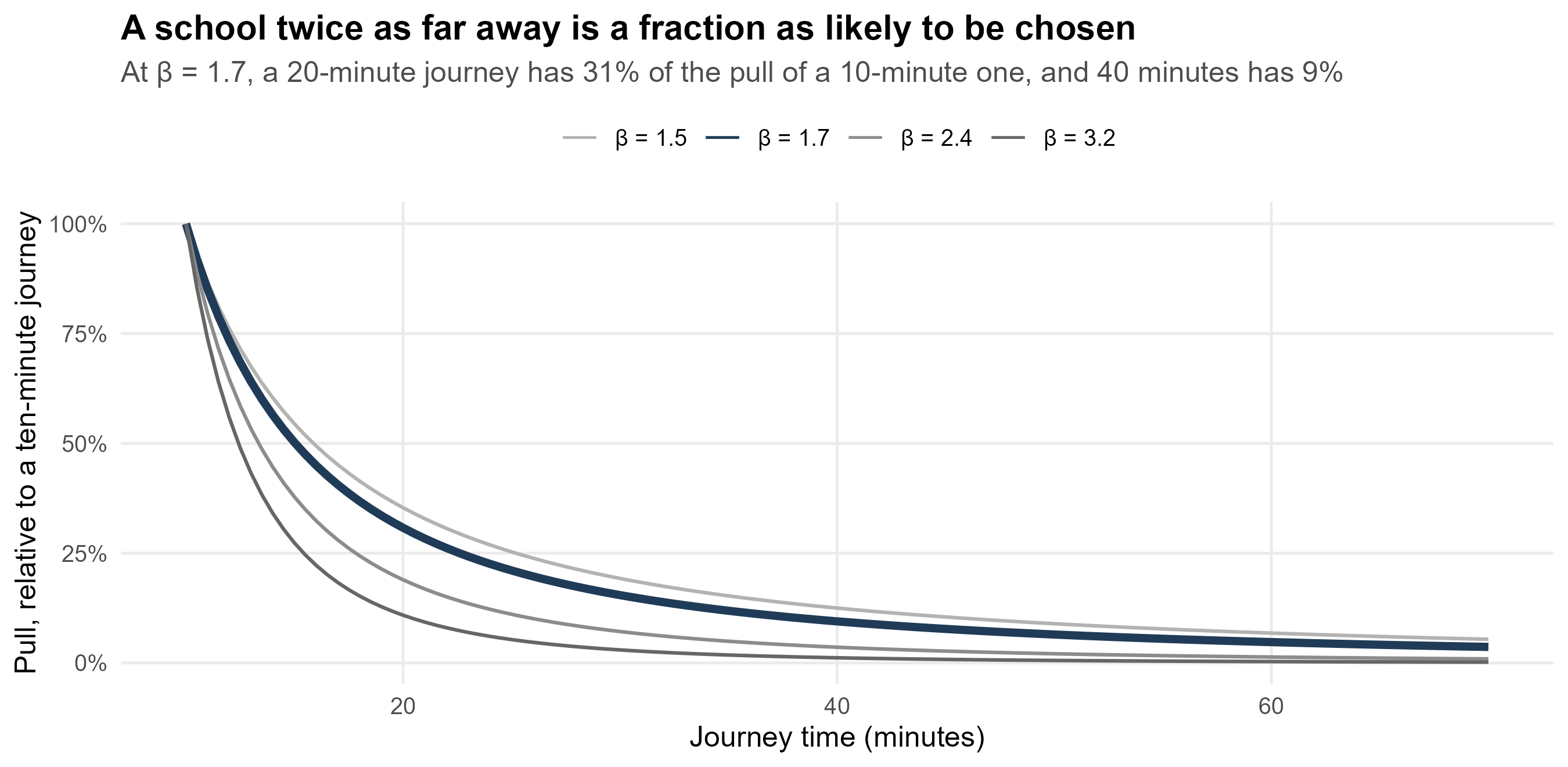
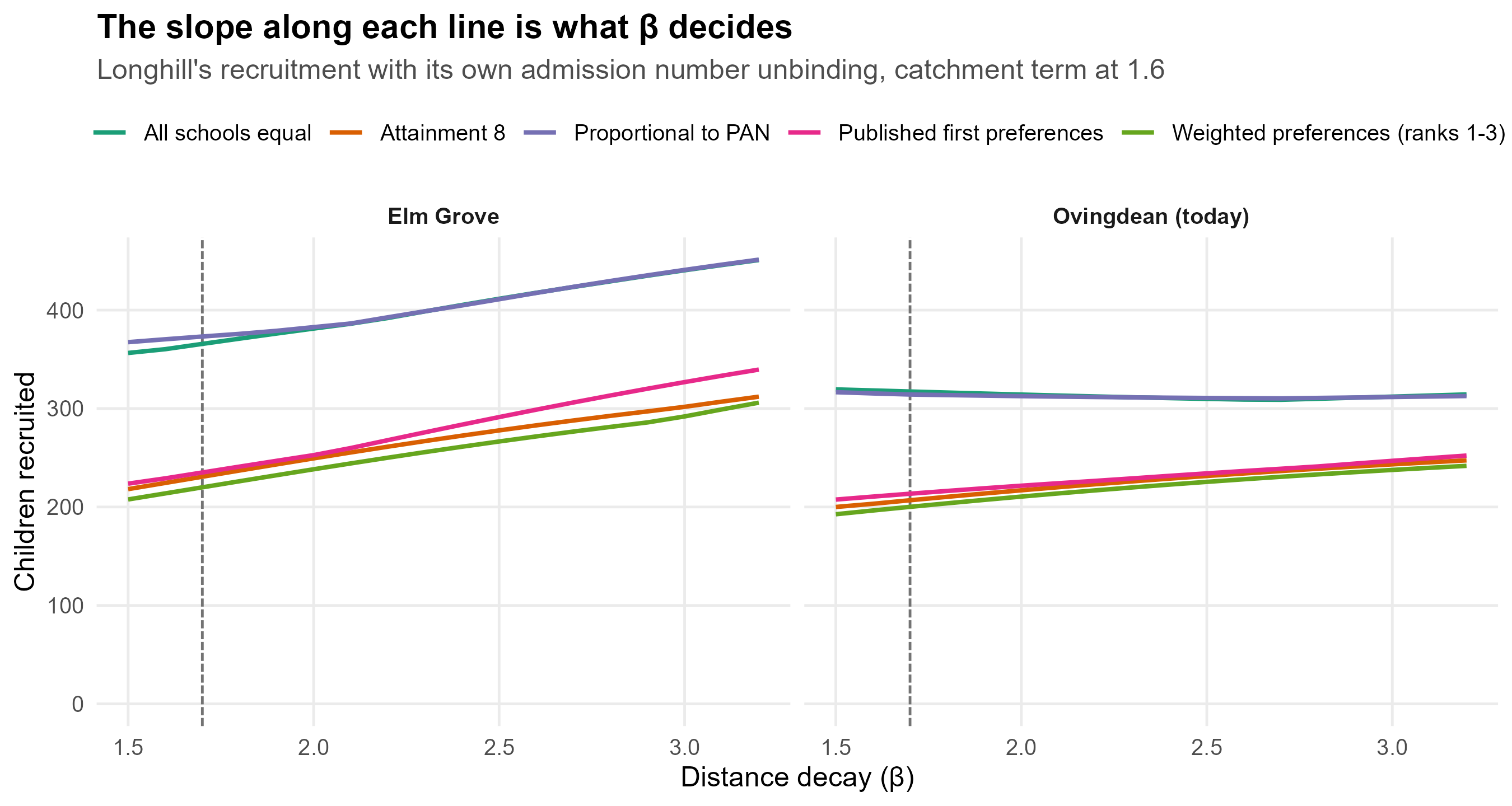
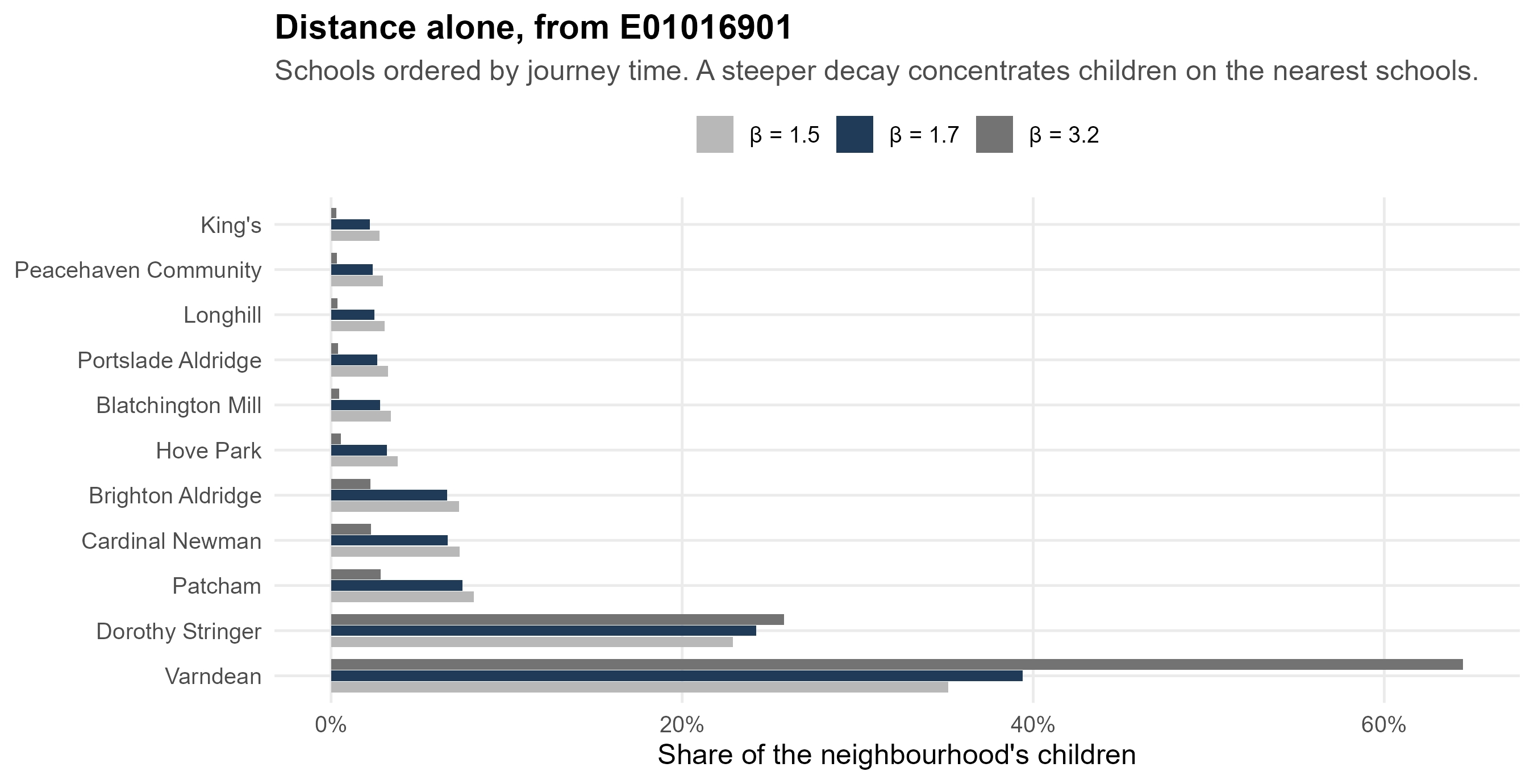
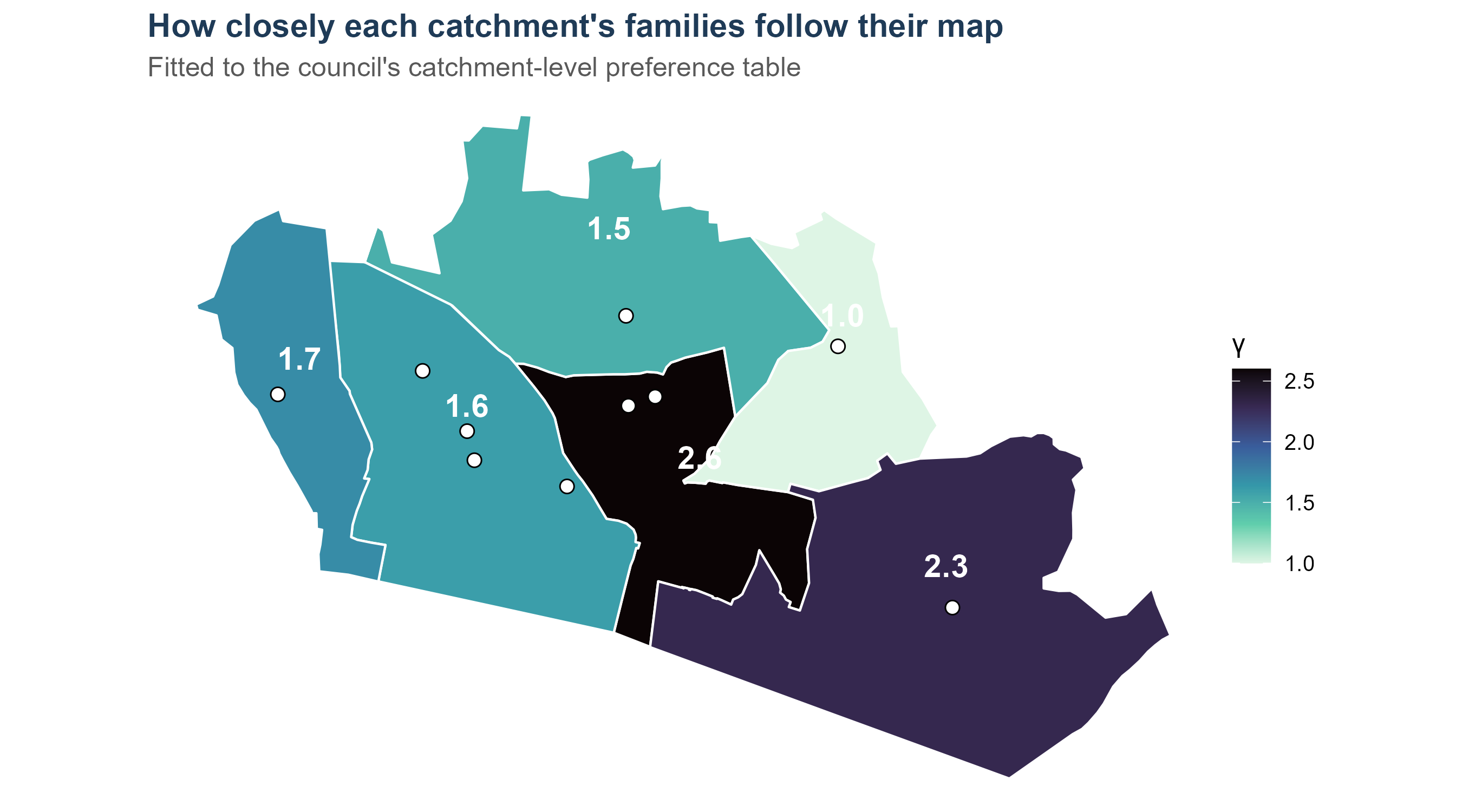
---
title: "The model, stage by stage"
subtitle: "A technical guide for checking each element"
author: "Adam Dennett, UCL Centre for Advanced Spatial Analysis"
date: today
abstract: |
This document takes the model the simulator runs and opens it up one
element at a time. Each section states what a term is, where its data
comes from, exactly how it is computed, what it looks like for a worked
example, the checks that can be run against it, and what it assumes. It
is written to be audited: every number is produced by the code in this
repository, and every step should be reproducible by hand.
---
```{r setup}
#| include: false
source(here::here("R", "00_core.R"))
library(scales)
knitr::opts_chunk$set(dev = "ragg_png", dpi = 150)
oi <- bh_data("open_inputs.rds")
mt <- bh_data("model_terms.rds")
inp <- readRDS(here::here("app", "data", "sim_inputs.rds"))
z <- oi$zones
zc <- z %>% filter(area != "Expansion area")
dem <- inp$demand
cal <- mt$calibrated
rc <- bh_data("reception_cohort.rds")
acc <- bh_data("accessibility.rds")
# The simulator's own engine, so the guide can run the model it describes.
source(here::here("app", "R", "model.R"))
source(here::here("app", "R", "outcomes.R"))
# The state-sector share is a single constant in the open bundle's build.
# It is recovered here from the projection rather than retyped, so this
# document cannot drift from the number the model used.
dem_raw <- readr::read_csv(here::here("data", "open_demand_projection.csv"),
show_col_types = FALSE)
STATE_SHARE <- with(dem_raw[dem_raw$area == "Brighton & Hove" &
dem_raw$entry_year == 2026, ],
state_demand / children)
W5 <- cal$W / mean(cal$W)
```
# What this document is
The simulator runs one model. Everything in the strategic view, and every
scenario in it, is that model with different settings. This guide takes
it apart in the order the model is written, so that each piece can be
checked on its own.
$$
T_{ij}^{\,y} \;=\; A_i^{\,y}\, O_i^{\,y}\, W_j\, c_{ij}^{-\beta}\,
e^{\gamma_{h(i)} \cdot \mathbb{1}[\,i \in \text{catchment}(j)\,]}\, C_j^{\delta},
\qquad
A_i^{\,y} = \frac{1}{\sum_k W_k\, c_{ik}^{-\beta}\, e^{\gamma_{h(i)} \mathbb{1}[\cdot]}\, C_k^{\delta}}
$$
| Symbol | Meaning | Section |
|:--|:--|:--|
| $T_{ij}$ | children from neighbourhood $i$ modelled as attending school $j$ | the interior of the matrix |
| $O_i$ | children in neighbourhood $i$ entering Year 7 | §2 |
| $W_j$ | how attractive school $j$ is, net of where it stands | §3 |
| $c_{ij}$ | routed walk-and-bus journey time from $i$ to $j$ | §4 |
| $\beta$ | distance decay | §5 |
| $\gamma_h$ | catchment term, fitted for each catchment $h$ | §6 |
| $C_j$, $\delta$ | competing destinations | §7 |
| $A_i$ | balancing factor: every neighbourhood places all of its children | §8 |
| $y$ | entry year, carried as a superscript | §2.7 |
Two further stages are applied to the $T_{ij}$ this produces: the
admission-number ceiling with the council's oversubscription priorities
(§9), and the re-offering of the children it refuses (§10).
::: {.callout-note}
## The year is the only dynamic element, and it enters in one place
Nothing in the equation carries a time subscript except $O_i$. Journey
times, attractiveness, catchment terms and admission numbers are all held
at a single point in time, and the year chosen on the simulator's slider
changes only the **size** of each neighbourhood's cohort (§2.7). Whether
that is the right treatment — and what an explicit time dimension would
have to carry — is a question this guide returns to once the static terms
are set out.
:::
```{r matrix-blank}
#| tbl-cap: "The shape of the model, for four neighbourhoods and four schools. Sections 2 and 3 fill in the two margins shown; the rest follow, and the interior cells come last."
ex_zones <- zc %>% arrange(desc(Oi)) %>% slice(1:4)
sch4 <- c("Dorothy Stringer School", "Varndean School",
          "Longhill High School", "Cardinal Newman Catholic School")
data.frame(
  Neighbourhood = c(sub("[|].*$", "", ex_zones$zone), "$W_j$"),
  `Dorothy Stringer` = c(rep("$T_{ij}$", 4), sprintf("%.2f", W5[[sch4[1]]])),
  Varndean = c(rep("$T_{ij}$", 4), sprintf("%.2f", W5[[sch4[2]]])),
  Longhill = c(rep("$T_{ij}$", 4), sprintf("%.2f", W5[[sch4[3]]])),
  `Cardinal Newman` = c(rep("$T_{ij}$", 4), sprintf("%.2f", W5[[sch4[4]]])),
  `$A_i$` = c(rep("?", 4), ""),
  `$O_i$ (2026)` = c(sprintf("%.1f", ex_zones$Oi), ""),
  check.names = FALSE) %>%
  knitr::kable(align = "lccccrr")
```
The interior of that matrix is what the model produces. The margins are
what it is given, or what it fits. $O_i$ is the one margin that is a
count of real people, and it is where this guide starts.
# $O_i$: the children in each neighbourhood {#sec-oi}
## What it is
$O_i$ is the number of children living in zone $i$ who will enter Year 7
at a **state** secondary school in the year being modelled. The model is
production-constrained on it, which means that whatever else happens,
$$\sum_j T_{ij} = O_i \quad \text{for every } i.$$
Every child is placed somewhere. Nothing is created and nothing is lost,
which is why $O_i$ has to be right before anything else can be.
## What a zone is
A zone is **an LSOA cut by catchment**, keyed as
`LSOA | pre-2024 catchment | current catchment`. The city has
`r fmt_n(nrow(zc))` zones drawn from `r fmt_n(n_distinct(zc$lsoa))`
LSOAs.
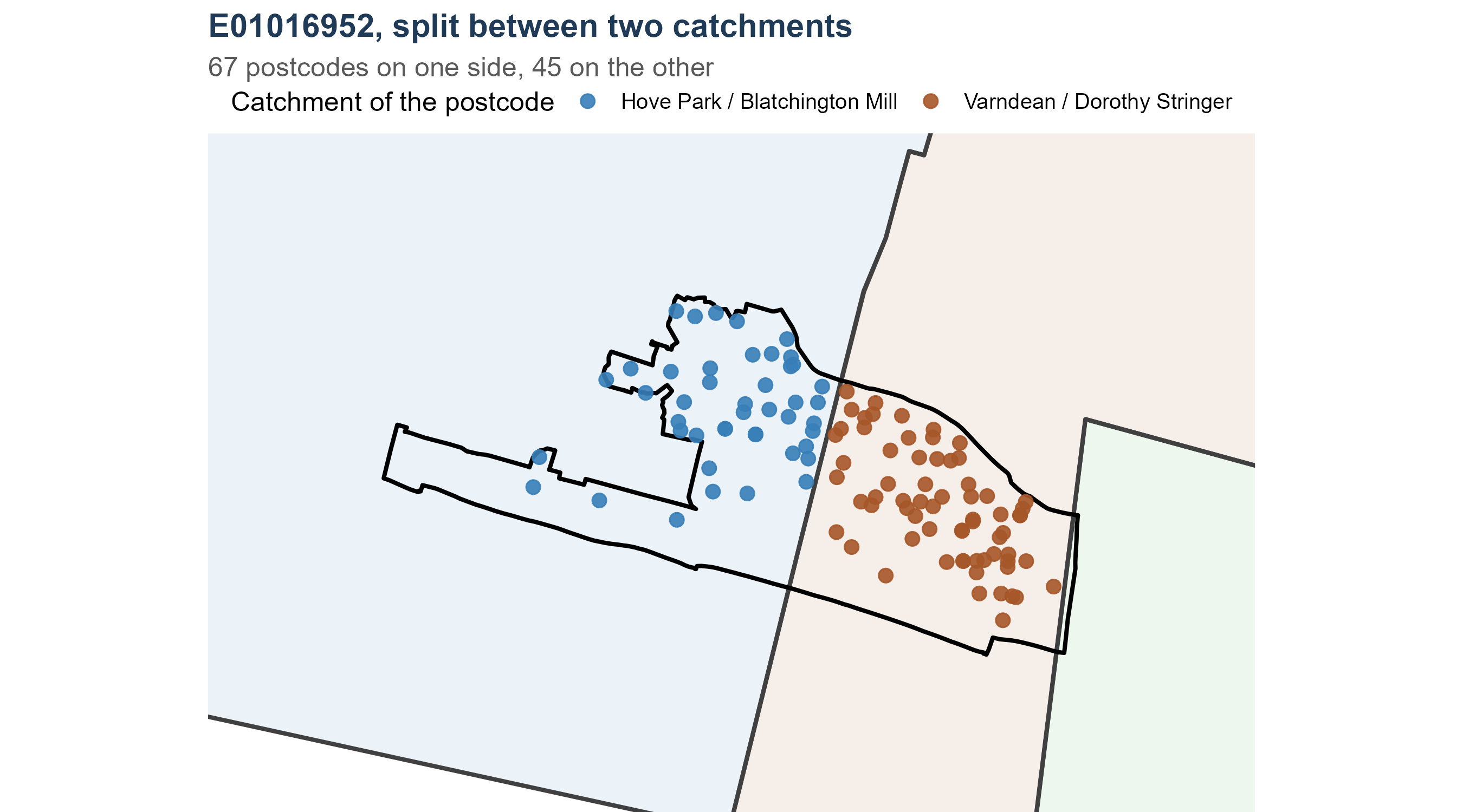
The cut exists because the 2024 boundary change runs *through* LSOAs.
Assigning a whole LSOA to whichever catchment contains its centroid would
register only a fraction of the children the redraw actually moves. So
every postcode in the ONS Postcode Directory is assigned a catchment on
each of the two maps by point-in-polygon, and the LSOA is split
accordingly. Carrying **both** maps in the key means the two regimes sit
on identical geography and can be compared without rebuilding anything.
```{r zone-example}
#| tbl-cap: "Two LSOAs on the Longhill / Stringer-Varndean boundary, each split into two zones: the same neighbourhood, a different catchment on the current map."
z %>%
  filter(lsoa %in% c("E01016862", "E01016863")) %>%
  transmute(Zone = zone, LSOA = lsoa, `Pre-2024` = catch_pre2024,
            `Current map` = catch_optionZ, Postcodes = n_pcd,
            `$O_i$ (2026)` = sprintf("%.1f", Oi)) %>%
  knitr::kable(align = "llllrr")
```
## Where the numbers come from {#sec-oi-sources}
| Input | Source | What it supplies |
|:--|:--|:--|
| Ward population by single year of age, mid-2022 | [ONS ward-level mid-year population estimates](https://www.ons.gov.uk/peoplepopulationandcommunity/populationandmigration/populationestimates/datasets/wardlevelmidyearpopulationestimatesexperimental) (`sapewardstablefinal.xlsx`) | how many children of each age live in each ward |
| LSOA population by single year of age | [ONS lower super output area mid-year population estimates](https://www.ons.gov.uk/peoplepopulationandcommunity/populationandmigration/populationestimates/datasets/lowersuperoutputareamidyearpopulationestimates) (`lsoa_age_11_props_totals.xlsx`) | how a ward's children divide between its LSOAs |
| Postcode directory, February 2024 | [ONS Postcode Directory, ONS Open Geography Portal](https://geoportal.statistics.gov.uk/) | which ward and LSOA each postcode is in |
| Catchment boundaries | [Brighton & Hove City Council, school admissions](https://www.brighton-hove.gov.uk/schools-and-learning/school-admissions) — the option Z map in force from 2026 entry, and the map it replaced | the catchment half of the zone key |
| Year 7 offers, 2024 | [Allocation factsheet, Year 7 places September 2024](https://www.brighton-hove.gov.uk/schools-and-learning/school-policies-reports-strategies-and-other-documents/allocation-factsheet-year-7-places-september-2024) | the state-sector share |
| LSOA boundaries | [ONS Open Geography Portal](https://geoportal.statistics.gov.uk/) | drawing, and joining the age data to zones |
None of it is pupil-level. The smallest thing any of these sources
describes is a postcode count or an LSOA age band.
## How $O_i$ is built, step by step
The code is `public/R/01_open_inputs.R` in the private bundle, sections
1b and 1c. Its result travels to the simulator as `data/open_inputs.rds`.
**Step 1 — ages become entry years.** A child aged $a$ in the mid-2022
estimates enters Year 7 in $2022 + (11 - a)$. Ages 0 to 11 therefore give
entry years 2022 to 2033, every one of them children ONS has already
counted rather than births anyone has projected.
**Step 2 — two extrapolated years.** Children entering in 2034 and 2035
were not born when the mid-2022 estimate was taken. They are a linear
continuation of the five most recent observed cohorts, 2029 to 2033, and
are flagged as extrapolated wherever they appear.
**Step 3 — resident children become state-sector demand.** Not every
resident child takes a state Year 7 place: some go to independent
schools, some leave the city. A single constant carries that:
$$\text{state share} \;=\; \frac{\text{Year 7 offers made, 2024}}{\text{resident children, 2024 entry}} \;=\; `r sprintf("%.3f", STATE_SHARE)`$$
taken from the council's published offer total against the ONS cohort of
the same year.
**Step 4 — a ward is divided between its zones.** ONS publishes the age
detail at ward level, so each ward's children are shared out between the
zones in it. The weight for a zone is its LSOA's age-11 population share,
divided between the zones that LSOA is cut into by their postcode counts:
$$u_i \;=\; \underbrace{p_{\ell(i)}}_{\text{LSOA age-11 share}} \times
\underbrace{\frac{n_i}{\sum_{k \in \ell(i)} n_k}}_{\text{postcodes in this zone}},
\qquad
O_i^{\,2026} \;=\; \text{ward children}_{w(i)} \times \frac{u_i}{\sum_{k \in w(i)} u_k} \times \text{state share}$$
where $\ell(i)$ is the zone's LSOA, $w(i)$ its ward and $n_i$ its
postcode count. `r fmt_n(sum(!is.na(z$prop)))` of the `r fmt_n(nrow(z))`
zones use the ONS age share; the `r fmt_n(sum(is.na(z$prop)))` in the
expansion area outside the city fall back to postcode counts alone.
::: {.callout-note appearance="simple"}
## Why not divide a ward by postcode count
Splitting a ward's children by how many postcodes each LSOA holds assumes
every postcode contains the same number of eleven-year-olds. Family
housing, student housing and retirement housing differ enormously on
that, and the difference runs along exactly the lines catchment
boundaries follow. An earlier version of this work used postcode counts
between LSOAs, and the deprivation contrast between the two halves of a
paired catchment was almost entirely smoothed away. Postcode counts do
the narrower job above — dividing one LSOA between its own fragments,
where nothing finer is published.
:::
::: {.callout-important}
## Corrected: a split LSOA used to be counted twice
Until this version, each zone of a split LSOA inherited the **whole**
LSOA's age-11 share as its weight. Ward and city totals were unaffected,
because the denominator grew too, but inside a ward a split LSOA took
about 1.7 to 1.9 times the share its population implied and the unsplit
LSOAs around it took correspondingly less. The splits sit exactly on the
catchment boundaries, so the error was concentrated in the neighbourhoods
these questions turn on — Whitehawk and Kemptown among them.
The weight is now divided between a split LSOA's zones by their postcode
counts, as in the formula above. The table below is the check that used
to fail.
:::
```{r split-check}
#| tbl-cap: "Each LSOA's modelled share of its ward against the share its age-11 population implies, grouped by how many zones the LSOA is split into. A ratio of 1 is agreement."
chk <- z %>% filter(!is.na(prop)) %>%
  group_by(ward) %>% mutate(zone_share = Oi / sum(Oi)) %>% ungroup() %>%
  group_by(ward, lsoa) %>%
  summarise(prop = first(prop), zone_share = sum(zone_share),
            n_zones = n(), .groups = "drop") %>%
  group_by(ward) %>% mutate(prop_share = prop / sum(prop)) %>% ungroup() %>%
  mutate(ratio = zone_share / prop_share)
chk %>%
  group_by(`Zones the LSOA is split into` = n_zones) %>%
  summarise(LSOAs = n(), `Median ratio` = sprintf("%.2f", median(ratio)),
            Lowest = sprintf("%.2f", min(ratio)),
            Highest = sprintf("%.2f", max(ratio)), .groups = "drop") %>%
  knitr::kable(align = "rrrrr")
```
`r fmt_n(sum(z$Oi[z$lsoa %in% chk$lsoa[chk$n_zones > 1]]))` of the
`r fmt_n(sum(z$Oi))` children in the model live in a split LSOA, so the
correction moves children between zones inside those wards without
changing any ward or city total.
```{r fig-split-lsoa}
#| fig-cap: "One LSOA cut by the catchment boundary in force from 2026. Each point is a live postcode, coloured by the catchment it falls in; the black line is the LSOA boundary and the heavier line the catchment boundary. The model splits the LSOA's children between the two sides in proportion to the postcodes on each."
#| fig-height: 5
pcd <- readr::read_csv(here::here("data", "zone_postcode_points.csv"),
                       show_col_types = FALSE)
# The clearest example to draw: the split LSOA with the most postcodes on
# its smaller side, so neither half is a handful of points.
pick <- pcd %>% count(lsoa, catch_optionZ) %>% group_by(lsoa) %>%
  filter(n() == 2) %>% summarise(smaller = min(n), .groups = "drop") %>%
  slice_max(smaller, n = 1) %>% pull(lsoa)
pp <- pcd %>% filter(lsoa == pick) %>%
  st_as_sf(coords = c("easting", "northing"), crs = 27700) %>% st_transform(4326) %>%
  mutate(Catchment = unname(CATCH_LABELS[as_boundary_catchment(catch_optionZ)]))
ls_one <- bh_data("lsoa.geojson") %>% filter(lsoa21cd == pick) %>% st_transform(4326)
catch_sf <- bh_data("catchments_current.geojson") %>% st_transform(4326)
bb <- st_bbox(st_buffer(st_transform(ls_one, 27700), 250)) %>%
  st_as_sfc() %>% st_transform(4326) %>% st_bbox()
ggplot() +
  geom_sf(data = catch_sf, aes(fill = catchment), colour = "grey25", alpha = 0.10,
          linewidth = 0.9, show.legend = FALSE) +
  geom_sf(data = ls_one, fill = NA, colour = "black", linewidth = 0.9) +
  geom_sf(data = pp, aes(colour = Catchment), size = 2.6, alpha = 0.9) +
  scale_fill_manual(values = CATCH_COLOURS) +
  scale_colour_manual(
    values = setNames(unname(CATCH_COLOURS[as_boundary_catchment(unique(pp$catch_optionZ))]),
                      unname(CATCH_LABELS[as_boundary_catchment(unique(pp$catch_optionZ))])),
    name = "Catchment of the postcode") +
  coord_sf(xlim = bb[c("xmin", "xmax")], ylim = bb[c("ymin", "ymax")]) +
  labs(title = sprintf("%s, split between two catchments", pick),
       subtitle = sprintf("%d postcodes on one side, %d on the other",
                          max(table(pp$catch_optionZ)), min(table(pp$catch_optionZ)))) +
  theme_void(12) +
  theme(plot.title = element_text(face = "bold", colour = "#1f3b57"),
        plot.subtitle = element_text(colour = "grey35"), legend.position = "top")
```
```{r split-worked}
#| tbl-cap: "The same LSOA, as the model sees it. The age-11 share belongs to the whole LSOA; each zone takes the part of it its postcodes imply."
z %>% filter(lsoa == pick) %>%
  transmute(Zone = zone, Postcodes = n_pcd,
            `Share of the LSOA` = sprintf("%.0f%%", 100 * n_pcd / sum(n_pcd)),
            `Age-11 share of the LSOA` = sprintf("%.4f", prop),
            `Weight used` = sprintf("%.4f", prop * n_pcd / sum(n_pcd)),
            `$O_i^{\\,2026}$` = sprintf("%.1f", Oi)) %>%
  knitr::kable(align = "lrrrrr")
```
Before the correction both rows of that table carried the whole LSOA's
age-11 share, so the neighbourhood counted twice in its ward's
denominator and took roughly double the children it should.
## A worked example
```{r oi-worked}
#| tbl-cap: "One ward, divided between its zones. Ward children is the ONS estimate for this cohort; the share is the zone's weight within the ward; O is the two multiplied together with the state-sector share."
wd <- z %>% filter(ward == (z %>% arrange(desc(Oi)) %>% slice(1) %>% pull(ward)))
wd %>%
  arrange(desc(Oi)) %>%
  transmute(Zone = sub("[|]", " | ", zone), LSOA = lsoa, Postcodes = n_pcd,
            `Age-11 share of LSOA` = sprintf("%.4f", prop),
            `Share of the ward` = sprintf("%.3f", share_in_ward),
            `Ward children` = fmt_n(ward_children),
            `$O_i$ (2026)` = sprintf("%.1f", Oi)) %>%
  knitr::kable(align = "llrrrrr")
```
Reading the first row: the ward holds `r fmt_n(wd$ward_children[1])`
children of this cohort; that zone carries
`r sprintf("%.1f%%", 100 * max(wd$share_in_ward))` of the ward's weight;
multiplied by the state-sector share of
`r sprintf("%.3f", STATE_SHARE)`, the zone holds
`r sprintf("%.1f", max(wd$Oi))` Year 7 children in 2026.
## The city total
```{r oi-total}
#| tbl-cap: "The modelled 2026 cohort by catchment. These are children living in the catchment, not children attending its school."
zc %>% group_by(Catchment = catchment) %>%
  summarise(children = sum(Oi), Zones = n(), .groups = "drop") %>%
  arrange(desc(children)) %>%
  transmute(Catchment, `Children, 2026` = fmt_n(children), Zones) %>%
  knitr::kable(align = "lrr")
```
The city's zones hold `r fmt_n(sum(zc$Oi))` children for 2026 entry. That
is the model's entire demand before any child chooses anything, and every
intake the simulator reports is drawn from it.
### Where the city totals come from {#sec-oi-provenance}
Two different city-wide totals appear in this work, and they have
different provenance. It is worth being explicit about which is which.
**Offers actually made** are the council's own published figures. Its
[allocation factsheets](https://www.brighton-hove.gov.uk/schools-and-learning/school-admissions)
are issued after each March allocation round, and the series from 2010 to
2026 was transcribed school by school in the earlier
[Brighton and Hove allocations](https://adamdennett.github.io/BH_Schools_2/brighton_and_hove_allocations.html)
analysis. This bundle does not retype them: `public/R/01a_factsheet_panel.R`
re-extracts the year-by-year tables from that document, so every offer,
preference and admission number here traces back to a published council
factsheet.
**Resident children** are ONS, as set out in @sec-oi-sources. They are a
different quantity from offers: a resident child may go to an independent
school, or out of the city.
**The model's city total is the first anchored on the second.** The
state-sector share of `r sprintf("%.3f", STATE_SHARE)` is the council's
published 2024 offer total divided by the ONS resident cohort for the same
entry year, so the model's demand is ONS children scaled to the level the
council's own offers imply. It is not a free-floating estimate.
```{r oi-provenance}
#| tbl-cap: "The two totals, and the model's demand between them."
fp <- bh_data("factsheet_panel.rds")$factsheets %>% filter(name != "Total")
off <- fp %>% group_by(year) %>% summarise(offers = sum(off_total), .groups = "drop")
tibble::tribble(
  ~Quantity, ~Source, ~Value,
  "Year 7 offers made, 2024", "Council allocation factsheet",
  fmt_n(off$offers[off$year == 2024]),
  "Year 7 offers made, latest round", "Council allocation factsheet",
  sprintf("%s (%d)", fmt_n(off$offers[which.max(off$year)]), max(off$year)),
  "Resident children, 2024 entry", "ONS ward estimates, mid-2022",
  fmt_n(dem_raw$children[dem_raw$area == "Brighton & Hove" & dem_raw$entry_year == 2024]),
  "State-sector share", "The first divided by the second",
  sprintf("%.3f", STATE_SHARE),
  "Model demand, 2026 entry", "ONS children x state share",
  fmt_n(sum(zc$Oi))) %>%
  knitr::kable(align = "llr")
```
The model's 2026 demand and the offers made in the 2026 round are not the
same number and should not be expected to match exactly: the offers
include children placed at a school they did not name, and exclude
children who took a place outside the city. The comparison is still worth
making, and it is the first check listed in @sec-oi-checks.
## The slider: how $O_i$ changes with the entry year {#sec-oi-year}
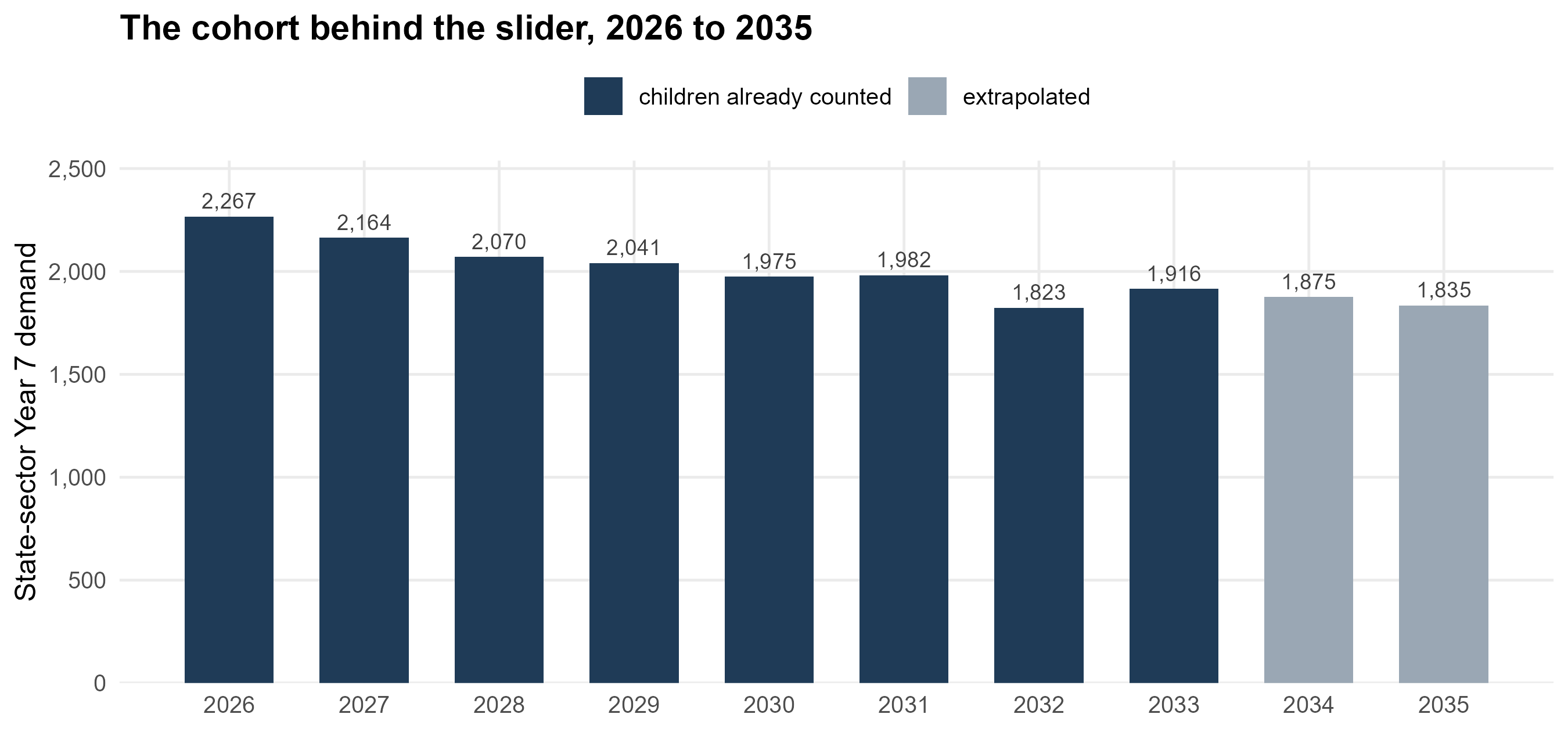
The year slider does exactly one thing to $O_i$. The city's projected
cohort is turned into an index on 2026, and every zone is scaled by it:
$$O_i^{\,y} \;=\; O_i^{\,2026} \times d^{\,y}, \qquad
d^{\,y} \;=\; \frac{\text{state demand}^{\,y}}{\text{state demand}^{\,2026}}$$
```{r oi-index}
#| tbl-cap: "The demand index behind the slider. The last two years are the extrapolated cohorts."
dem %>%
  transmute(`Entry year` = year, `City cohort` = fmt_n(cohort),
            `Index on 2026` = sprintf("%.3f", index),
            Basis = ifelse(extrapolated, "extrapolated",
                           "children already counted")) %>%
  knitr::kable(align = "rrrl")
```
```{r fig-oi-index}
#| fig-cap: "The cohort the model scales to. Every zone is multiplied by the same factor, so the map of where children live is held still and only the size of the cohort moves."
#| fig-height: 4.2
dem %>%
  ggplot(aes(year, cohort)) +
  geom_col(aes(fill = extrapolated), width = 0.66) +
  geom_text(aes(label = fmt_n(cohort)), vjust = -0.5, size = 3.2, colour = "grey25") +
  scale_fill_manual(values = c(`FALSE` = "#1f3b57", `TRUE` = "#9aa7b4"),
                    labels = c(`FALSE` = "children already counted",
                               `TRUE` = "extrapolated"), name = NULL) +
  scale_x_continuous(breaks = dem$year) +
  scale_y_continuous(labels = label_comma(), expand = expansion(mult = c(0, 0.12))) +
  labs(x = NULL, y = "State-sector Year 7 demand",
       title = "The cohort behind the slider, 2026 to 2035") +
  theme_bh() + theme(legend.position = "top")
```
### Which projection this is, and the one beside it {#sec-oi-projection}
Two projections of the city's Year 7 cohort appear in this work. They are
built from different data and they are used for different things, so it
is worth being plain about which drives the model.
**The one the slider uses** is the ONS estimate carried forward: the
children counted in the mid-2022 small-area estimates, aged forward to
their Year 7 entry year (§2.4, steps 1 and 2), and multiplied by the
state-sector share. It is used because it is the only one that exists at
**ward** level, and the model needs the geography as well as the total —
$O_i$ is a ward figure divided between zones.
**The one beside it** is built from children already in the city's
primary schools: Reception offers made seven years earlier, multiplied by
the share of a Reception cohort that reappears as a Year 7 offer. That
ratio is measured rather than assumed, from the council's own published
factsheets, and it has been strikingly steady —
`r fmt_pct(100 * rc$survival_recent, 1)` across the five most recent
cohorts, with a standard deviation of
`r fmt_pct(100 * rc$survival_sd, 1)`. The method is set out in full in
[how our projection method works](https://adamdennett.github.io/BH_Schools_2/brighton_and_hove_allocations.html#how-our-projection-method-works),
and section 3 of the strategic view uses it as its headline projection
because it rests on children already registered in a school rather than
on a population estimate.
```{r oi-two-projections}
#| tbl-cap: "The two projections side by side. The first drives the model's zone-level demand; the second is the check on it, and the strategic view's headline series."
rc$comparison %>%
  transmute(`Entry year` = entry_year,
            `From ONS estimates (drives the slider)` = fmt_n(ons_demand),
            `From Reception offers` = fmt_n(reception_based),
            Difference = sprintf("%+.0f", reception_based - ons_demand),
            `%` = sprintf("%+.1f%%", 100 * (reception_based / ons_demand - 1))) %>%
  knitr::kable(align = "rrrrr")
```
They agree within a few per cent for most years, which is reassuring for
both, and they diverge most in the years where the ONS series is itself
extrapolated. Neither is a forecast in the sense of predicting behaviour:
one counts children who exist, the other counts children already in
school and applies a measured survival rate.
**What this does not do.** The projection is city-wide, so the slider
cannot say that one neighbourhood shrinks faster than another: every zone
keeps its 2026 share of the city's children in every year. The council's
own forecasts differ from this mostly in exactly that respect — its
Longhill catchment line falls faster than the city's does — so comparing
catchment totals year by year compares two different claims rather than
two estimates of one thing.
## Checks you can run {#sec-oi-checks}
```{r oi-checks}
#| tbl-cap: "Identities that should hold, and what they give as this document is built."
ward_tot <- z %>% group_by(ward) %>%
  summarise(oi = sum(Oi), implied = first(ward_children) * STATE_SHARE,
            .groups = "drop") %>%
  mutate(d = abs(oi - implied))
tibble::tribble(
  ~Check, ~Result,
  "Every zone has a positive cohort",
  sprintf("smallest is %.2f children", min(z$Oi)),
  "Zone cohorts sum to each ward's estimate times the state share",
  sprintf("largest difference %.3f children", max(ward_tot$d)),
  "The city's zones sum to the 2026 projection",
  sprintf("%s against %s", fmt_n(sum(zc$Oi)), fmt_n(dem$cohort[dem$year == 2026])),
  "The index is exactly 1 in the base year",
  sprintf("%.6f", dem$index[dem$year == 2026]),
  "A split LSOA takes the share its population implies",
  sprintf("largest ratio %.2f", max(chk$ratio))) %>%
  knitr::kable(align = "lr")
```
Two further comparisons are worth doing by hand, because they test $O_i$
against something the model never saw: the city total against the
council's published Year 7 offers for the same round, and each
catchment's total against the catchment forecasts in the council's place
planning appendix.
## Checked against the council's own count {#sec-oi-ward-check}
```{r oi-ward-setup}
#| include: false
wv <- bh_data("ward_validation.rds")
wv_r <- cor(wv$compare$modelled, wv$compare$ks2)
wv_fit <- wv$fit
wv_lo <- wv$shares %>% slice_min(share, n = 1)
wv_hi <- wv$shares %>% slice_max(share, n = 1)
```
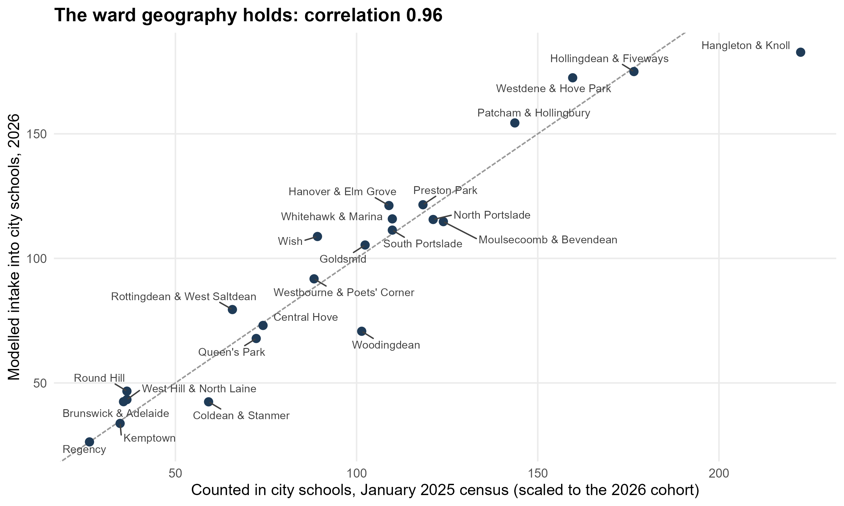
Everything above tests $O_i$ against its own ingredients. The council's
Educational Equity Framework makes an external test possible for the
first time: its Appendix 1 counts Key Stage 2 and Key Stage 4 pupils by
home ward, assigned from the January 2025 school census. The Key Stage 2
count is Year 6 in that census — the children who entered Year 7 the
following September, which is the cohort this term is about. Its
lineage shares nothing with ours: census home addresses, against our ONS
mid-year estimates.
One feature of the table decides how it must be used. It counts pupils
**in Brighton & Hove schools**. Residents at independent schools, at
schools in other authorities, at non-maintained special schools,
educated at home or solely registered at a pupil referral unit are all
absent from it. So the right comparison is not against $O_i$, which also
holds the children the model sends to Priory, Peacehaven, Seahaven and
Seaford Head, but against modelled flows *into city schools* by home
ward. The council's cohort is a year earlier and about 6% larger than
the 2026 one, so what is compared is the shape: each ward's modelled
intake against its counted intake, after that city-wide difference is
divided out.
```{r oi-ward-chart}
#| fig-height: 5.4
#| fig-cap: "Modelled intake into city schools against the council's count, by home ward. A ward above the line is one the model sends to city schools in greater numbers than the census found there."
wv$compare %>%
  mutate(ward = forcats::fct_reorder(ward, ratio)) %>%
  ggplot(aes(expected, modelled)) +
  geom_abline(slope = 1, intercept = 0, colour = "grey60", linetype = "31") +
  geom_point(colour = "#1f3b57", size = 2.6) +
  ggrepel::geom_text_repel(aes(label = ward), size = 3, colour = "grey25",
                           seed = 4, max.overlaps = 20, box.padding = 0.45) +
  scale_x_continuous(labels = label_comma()) +
  scale_y_continuous(labels = label_comma()) +
  labs(x = "Counted in city schools, January 2025 census (scaled to the 2026 cohort)",
       y = "Modelled intake into city schools, 2026",
       title = sprintf("The ward geography holds: correlation %.2f", wv_r)) +
  theme_bh()
```
The geography is sound. What the residuals show is the assumption the
previous page warned about: the single state-sector share. Rebuilding
each ward's children so that modelled city intakes match the counted
ones — holding the city total fixed, so the council's projection still
sets the level — implies a share that is anything but flat.
```{r oi-ward-shares}
#| tbl-cap: "The share of each ward's ONS children implied by the council's count, against the flat share the model uses. Above 1.0 means the ONS estimate is too low for that ward, not that every child attends a city school."
wv$shares %>%
  transmute(Ward = ward,
            `ONS children` = fmt_n(ward_children),
            `Counted (KS2)` = fmt_n(ks2),
            `Implied share` = sprintf("%.2f", share),
            `Against the flat %.2f` = sprintf("%+.0f%%", 100 * (vs_flat - 1))) %>%
  rlang::set_names(c("Ward", "ONS children", "Counted (KS2)", "Implied share",
                     sprintf("Against the flat %.2f", wv$flat_share))) %>%
  knitr::kable(align = "lrrrr")
```
It runs from `r sprintf("%.2f", wv_lo$share)` in `r wv_lo$ward` to
`r sprintf("%.2f", wv_hi$share)` in `r wv_hi$ward`. The low end is where
independent-school take-up is heaviest and, in Rottingdean & West
Saltdean, where children also cross the boundary eastwards. The values
above one mean the ONS ward estimate is too low, so the model has been
carrying too few children in Hangleton & Knoll and Coldean & Stanmer.
The test of whether this is a correction rather than a rearrangement is
the published offers, which play no part in deriving the shares:
```{r oi-ward-fit}
#| tbl-cap: "The same model, run on per-ward shares, against the offers Brighton & Hove schools made for September 2026."
wv_fit %>%
  transmute(Origins = c("current" = "One share for the whole city",
                        "per_ward" = "A share for each ward")[origins],
            `R²` = sprintf("%.3f", r2),
            `Root mean square error` = sprintf("%.1f", rmse),
            `Mean absolute error` = sprintf("%.1f", mae)) %>%
  knitr::kable(align = "lrrr")
```
The fit improves on every measure, and it improves at the schools where
the model is furthest out: Patcham comes down from
`r sprintf("%.0f", wv$intakes$current[wv$intakes$name == "Patcham High School"])`
to `r sprintf("%.0f", wv$intakes$per_ward[wv$intakes$name == "Patcham High School"])`
against an observed `r fmt_n(wv$intakes$observed[wv$intakes$name == "Patcham High School"])`,
and Brighton Aldridge rises from
`r sprintf("%.0f", wv$intakes$current[wv$intakes$name == "Brighton Aldridge Community Academy"])`
to `r sprintf("%.0f", wv$intakes$per_ward[wv$intakes$name == "Brighton Aldridge Community Academy"])`,
still short of its observed `r fmt_n(wv$intakes$observed[wv$intakes$name == "Brighton Aldridge Community Academy"])`
but less so.
One caution about what the shares mean. For Woodingdean the counted
intake is well above the modelled one, and the fix raises the ward's
children by about 40%. That is one of two things, and this table cannot
tell them apart: either the ONS estimate is too low there, or the model
sends too many Woodingdean children out of the city to Priory and
Peacehaven. Both would show up the same way. The adjustment corrects the
arithmetic either way, but only the first is a statement about how many
children live there.
**This is not yet in the model the simulator runs.** The results in this
guide, in the strategic view and in the simulator all use the flat share.
Changing it rebuilds every number in every document, which is a decision
to take deliberately rather than as a side effect of a validation
section. What the section establishes is that the origins are sound in
shape, that the flat share is the largest remaining error in them, and
that the correction is available and improves the fit.
## What to be careful about
- **The base is mid-2022.** Migration into or out of the city since then
is not in the counts, and a child who has moved between wards is still
counted where they were.
- **One state-sector share, for every year and every neighbourhood.** It
is `r sprintf("%.3f", STATE_SHARE)`, from a single round. If
independent-school take-up varies across the city — and it plainly does
— then $O_i$ is too high in some places and too low in others.
- **Ward-level age detail.** Within a ward, the LSOA age-11 distribution
does the work; how children are distributed inside an LSOA is not
observed, so postcode counts stand in for it where a boundary cuts one.
- **Peacehaven and the expansion area** are carried in the open bundle
but excluded from the simulator's zones. Peacehaven Community School is
a destination in the model, not a source of demand.
- **No composition.** $O_i$ is a headcount. Which of those children are
disadvantaged is a separate layer applied later, not part of this term.
## Questions this raises
1. Should the state-sector share vary by neighbourhood, given that
independent-school take-up does?
2. Should the year slider move the *geography* of demand as well as its
size — that is, should each catchment carry its own projection, as the
council's forecasts do?
# $W_j$: how attractive each school is {#sec-wj}
## What it is
$W_j$ is the pull of school $j$ on a family, **net of where the school
stands**. It is dimensionless, scaled so the city average is 1, and it
enters the model multiplicatively: doubling $W_j$ doubles the numerator
of every flow into $j$ before distance, catchment and competition have
their say. It also enters the competing-destinations term, because a
school's rivals count for more when they are schools families want.
It is the hardest term in the model to pin down, because everything
observable about a school is entangled with where it is. A school with
high attainment may be sought after because it teaches well, or because
it sits where better-off families already live.
## Two layers: the open specifications, and the fitted values
**Layer one — the open specifications.** The open bundle carries five
candidate measures of attractiveness, so that a conclusion can be tested
across all of them rather than resting on one.
```{r wj-specs}
#| tbl-cap: "The five open specifications, each scaled so the city average is 1. Weighted preferences count ranks 1 to 3, a second preference worth half a first and a third a quarter."
oi$attract %>%
  transmute(School = short_sch(name), PAN = pan, `Attainment 8` = round(att8, 1),
            Equal = sprintf("%.2f", W_equal), `By PAN` = sprintf("%.2f", W_pan),
            `First preferences` = sprintf("%.2f", W_prefs),
            `Weighted preferences` = sprintf("%.2f", W_wprefs),
            `By Attainment 8` = sprintf("%.2f", W_att8)) %>%
  arrange(desc(as.numeric(`Weighted preferences`))) %>%
  knitr::kable(align = "lrrrrrrr")
```
The central one is **weighted preferences per place**: the council's
published factsheets, pooled over the most recent rounds, counting first,
second and third preferences with a geometric discount of 0.5 per rank,
divided by the admission number. The paired catchments are why: a family
in Stringer / Varndean or Hove Park / Blatchington Mill must rank two
local schools against each other, so a first-preference count reads a
school families put second as one nobody wanted.
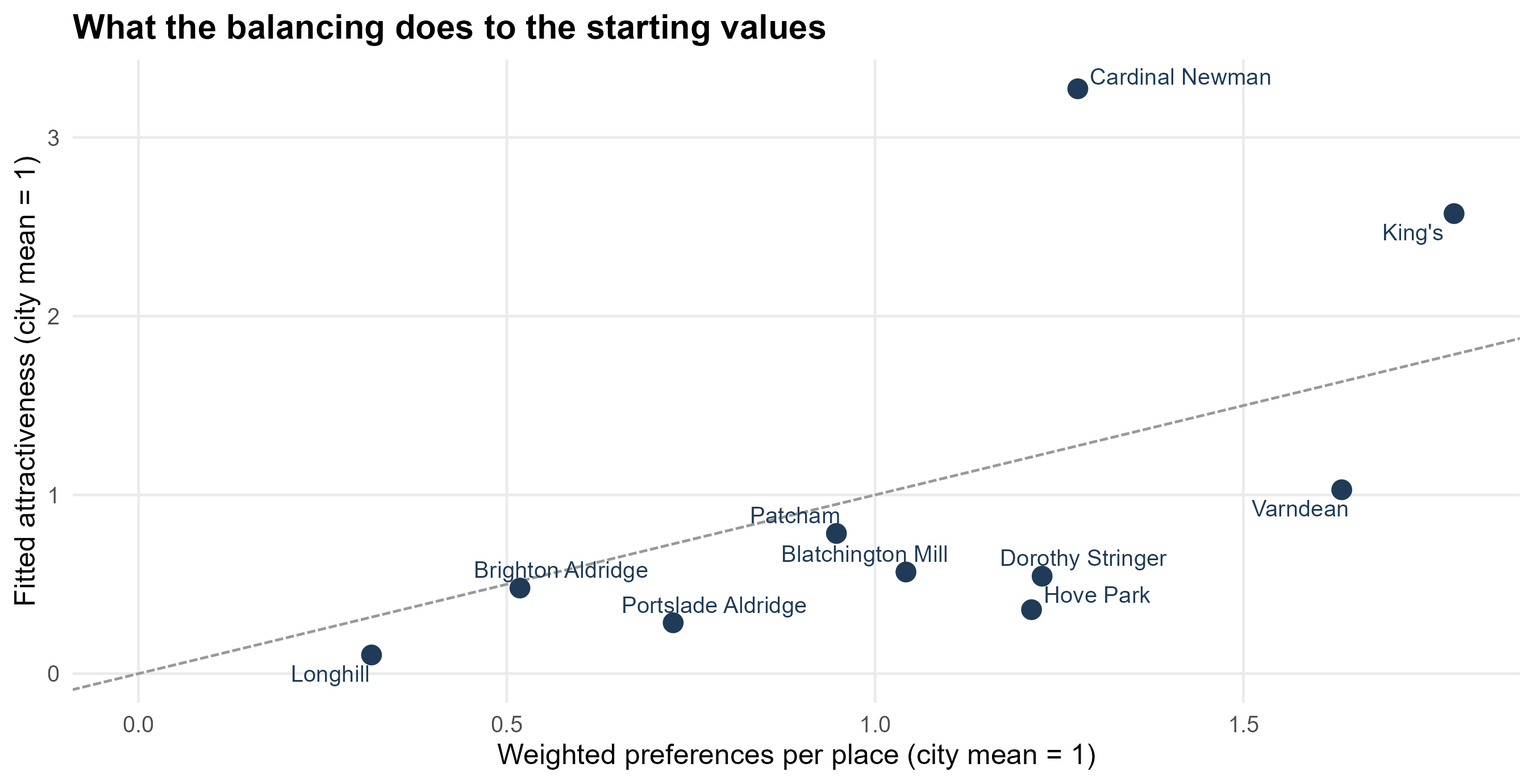
**Layer two — the fitted values the simulator uses.** The full model does
not take any of those five as given. It **balances** $W_j$ so that the
model reproduces the share of the city's first preferences each school
actually receives, using the council's catchment-level preference table
from its evidence to the Schools Adjudicator. The catchment terms
$\gamma_h$ are fitted in the same loop (§6), because the two
trade off against each other.
$$W_j \;\leftarrow\; W_j \left(\frac{\text{target share}_j}{\text{modelled share}_j}\right)^{0.8},
\qquad \text{repeat until } \max_j |\text{modelled} - \text{target}| < 10^{-6}$$
starting from the weighted-preference values, with the result rescaled to
a city mean of 1. The exponent 0.8 is damping: it stops the balancing
oscillating around the target. This is the same device as the balancing
factor $A_i$, applied to the other margin of the matrix — $A_i$ makes
every neighbourhood place all its children, and this makes every school
receive the share of first preferences it is observed to receive.
```{r wj-fitted}
#| tbl-cap: "The fitted attractiveness the simulator's sliders multiply, beside the weighted-preference measure it starts from, and each school's target share of the city's first preferences."
tibble(name = names(W5), W5 = as.numeric(W5)) %>%
  left_join(oi$attract %>% select(name, W_wprefs, att8), by = "name") %>%
  left_join(tibble(name = names(cal$target_first_prefs),
                   target = as.numeric(cal$target_first_prefs)), by = "name") %>%
  arrange(desc(W5)) %>%
  transmute(School = short_sch(name),
            `Weighted preferences` = sprintf("%.2f", W_wprefs),
            `Fitted $W_j$` = sprintf("%.2f", W5),
            `Target share of first preferences` = sprintf("%.1f%%", 100 * target),
            `Attainment 8` = sprintf("%.1f", att8)) %>%
  knitr::kable(align = "lrrrr")
```
```{r fig-wj}
#| fig-cap: "The fitted attractiveness against the measure it starts from. A school above the line is one the model has to make more attractive than its weighted preferences suggest to reproduce the preferences each catchment gives it."
#| fig-height: 4.6
tibble(name = names(W5), W5 = as.numeric(W5)) %>%
  left_join(oi$attract %>% select(name, W_wprefs), by = "name") %>%
  ggplot(aes(W_wprefs, W5)) +
  geom_abline(slope = 1, intercept = 0, colour = "grey60", linetype = "31") +
  geom_point(size = 3.4, colour = "#1f3b57") +
  ggrepel::geom_text_repel(aes(label = short_sch(name)), size = 3.4, seed = 1,
                           colour = "#1f3b57") +
  expand_limits(x = 0, y = 0) +
  labs(x = "Weighted preferences per place (city mean = 1)",
       y = "Fitted attractiveness (city mean = 1)",
       title = "What the balancing does to the starting values") +
  theme_bh()
```
## What point in time does $W_j$ belong to? {#sec-wj-time}
$W_j$ is **fixed**. One number per school, no year subscript, used for
2026 and for 2035 alike. That deserves stating plainly, because it is the
assumption a reader is least likely to notice and the one that a school
can falsify fastest.
Two windows go into it:
```{r wj-window}
#| tbl-cap: "The observations behind the attractiveness term."
fp <- bh_data("factsheet_panel.rds")
tibble::tribble(
  ~Layer, ~Source, ~Window,
  "Starting values: weighted preferences per place",
  "Council allocation factsheets",
  sprintf("%d rounds, %d onwards", fp$pref_years, fp$attract_from),
  "Fitted values: balanced to first preferences",
  "Council's catchment-level preference table",
  sprintf("%d rounds, %s", length(cal$rounds), paste(cal$rounds, collapse = ", ")),
  "Rank discount inside the window",
  "A second preference counts this much of a first",
  sprintf("%.2f, and a third %.2f", fp$wpref_decay, fp$wpref_decay^2)) %>%
  knitr::kable(align = "lll")
```
So the model's attractiveness describes the city as families have treated
it over the last three to five admissions rounds. It is a recent average,
not a long-run constant, and not a snapshot of one year either — a single
round moves too much to fit to.
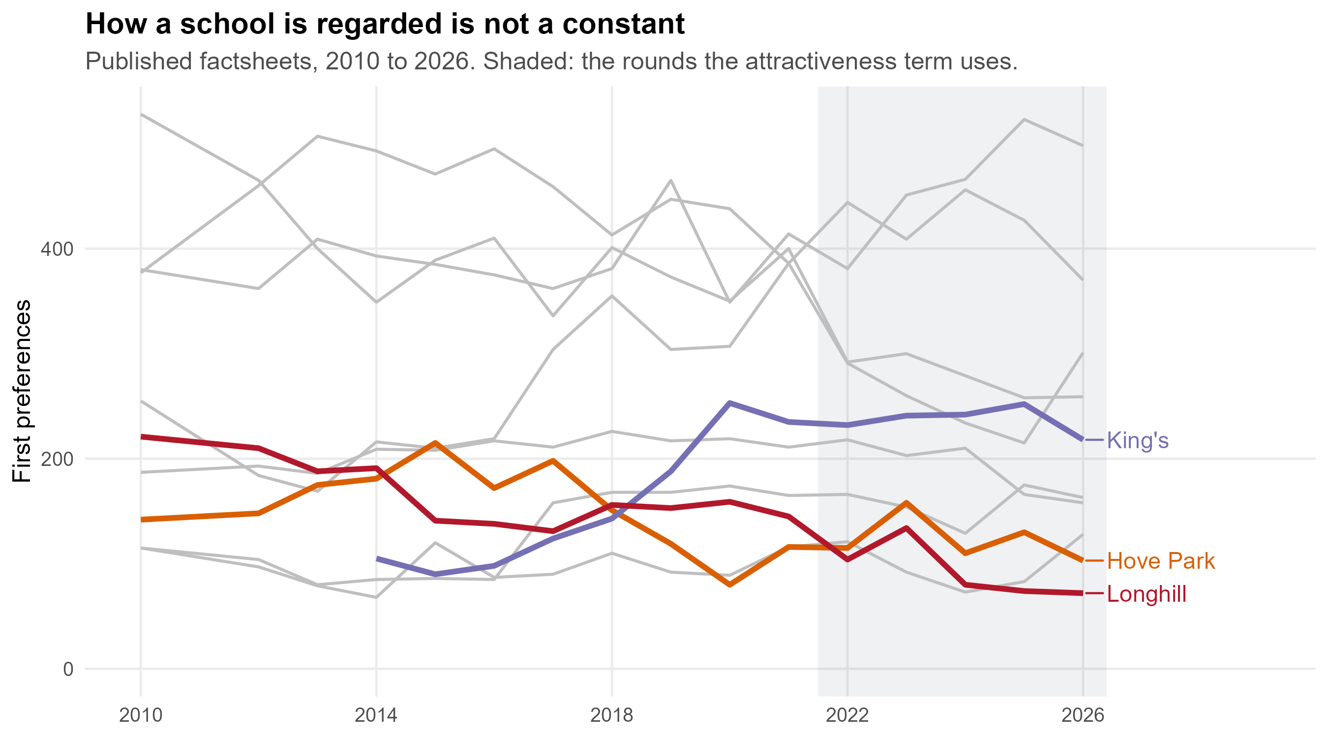
**Why that matters: the ordering is not stable over a decade.**
```{r fig-wj-time}
#| fig-cap: "First preferences for each school, from the published allocation factsheets. Nothing here is modelled. The shaded band is the window the attractiveness term is built from."
#| fig-height: 5
fs <- fp$factsheets %>% filter(name != "Total") %>%
  mutate(School = short_sch(name),
         hl = School %in% c("King's", "Hove Park", "Longhill"))
ggplot(fs, aes(year, pref1, group = School)) +
  annotate("rect", xmin = fp$attract_from - 0.5, xmax = max(fs$year) + 0.4,
           ymin = -Inf, ymax = Inf, fill = "#1f3b57", alpha = 0.07) +
  geom_line(data = fs %>% filter(!hl), colour = "grey75", linewidth = 0.7) +
  geom_line(data = fs %>% filter(hl), aes(colour = School), linewidth = 1.3) +
  ggrepel::geom_text_repel(
    data = fs %>% filter(hl, year == max(year)), aes(label = School, colour = School),
    hjust = 0, nudge_x = 0.4, direction = "y", size = 4, seed = 2, show.legend = FALSE) +
  scale_colour_manual(values = c(`King's` = "#7570b3", `Hove Park` = "#d95f02",
                                Longhill = "#b2182b"), guide = "none") +
  scale_x_continuous(breaks = seq(2010, 2026, 4), limits = c(2010, 2029)) +
  expand_limits(y = 0) +
  labs(x = NULL, y = "First preferences",
       title = "How a school is regarded is not a constant",
       subtitle = sprintf("Published factsheets, %d to %d. Shaded: the rounds the attractiveness term uses.",
                          min(fs$year), max(fs$year))) +
  theme_bh()
```
Over sixteen years King's first preferences roughly doubled while Hove
Park's roughly halved, in the same part of the same city. A $W_j$ built
from 2014 would put those two schools the other way round from a $W_j$
built from 2026. Reputations move, and they can move quickly: a new head,
a turn in attendance or results, a building programme, an Ofsted
judgement.
::: {.callout-important}
## How the model handles this, and what it cannot do
**What it does.** It fixes attractiveness at its recent value and gives
you a slider to move it. Every scenario in the strategic view that says
"a school half as attractive again" is that slider, and §3.6 converts a
slider position into points of Attainment 8 so the size of the
assumption is legible rather than abstract.
**What it does not do.** Attractiveness never responds to anything the
model itself produces. A school whose roll falls does not become less
wanted in the next year of the run; a school whose intake changes does
not see its results, and therefore its reputation, move with it. The
feedback loop the strategic view describes — a more disadvantaged intake,
lower headline scores, fewer preferences, a more disadvantaged intake
still — is **outside** this model. Where that loop is real, a run over ten
years understates how far apart schools drift.
That is the clearest case in this document for making time explicit
rather than implicit: $O_i$ already carries a year, and the natural next
step would be to let $W_j$ carry one too.
:::
## Why there is no exponent on $W_j$ {#sec-wj-alpha}
The general form of a production-constrained model carries a power on
attractiveness as well as on cost:
$$T_{ij} \;=\; A_i\, O_i\, W_j^{\alpha}\, c_{ij}^{-\beta}$$
Here $\alpha$ is absent, which is the same as fixing it at 1. That is a
deliberate choice and it follows from what $W_j$ is.
**A fitted quantity does not need a parameter to scale it.** $W_j$ is not
a proxy standing in for attractiveness; it *is* attractiveness, balanced
until the model reproduces each school's share of the city's first
preferences. An exponent on it would be a second free parameter doing the
same job as the balancing, and the two would trade off against each other:
any $\alpha$ can be absorbed by re-balancing $W$, because
$(W^{1/\alpha})^{\alpha} = W$. Fitting both would be fitting the same
thing twice, and the pair would not be identified.
**It would be needed if $W_j$ were a proxy.** Suppose attractiveness were
taken crudely as the number of pupils on roll, or as the admission
number, or as Attainment 8 — all of which this work carries as
alternative specifications (§3.2). None of those *is* pull; each is a
measurable thing believed to move with it, and there is no reason the
relationship should be one-for-one. A school twice the size is not
necessarily twice as wanted. An exponent would then be exactly the right
device: $\alpha$ fitted to observed flows would say how strongly demand
responds to the proxy, and $\alpha = 1$ would be a finding rather than an
assumption. In the classic retail application that is precisely what the
exponent on floorspace does.
So the rule is: **balance it, or scale it, but not both.** This model
balances. A version of it built on roll or on published attainment, which
is what anyone without the council's preference table would have to do,
should carry an $\alpha$ and fit it.
## Where it sits in the matrix
```{r matrix-wj}
#| tbl-cap: "The same four neighbourhoods and schools. Two margins are now filled: the children in each neighbourhood, and the pull of each school."
data.frame(
  Neighbourhood = c(sub("[|].*$", "", ex_zones$zone), "$W_j$"),
  `Dorothy Stringer` = c(rep("$T_{ij}$", 4), sprintf("%.2f", W5[[sch4[1]]])),
  Varndean = c(rep("$T_{ij}$", 4), sprintf("%.2f", W5[[sch4[2]]])),
  Longhill = c(rep("$T_{ij}$", 4), sprintf("%.2f", W5[[sch4[3]]])),
  `Cardinal Newman` = c(rep("$T_{ij}$", 4), sprintf("%.2f", W5[[sch4[4]]])),
  `$A_i$` = c(rep("?", 4), ""),
  `$O_i$ (2026)` = c(sprintf("%.1f", ex_zones$Oi), ""),
  check.names = FALSE) %>%
  knitr::kable(align = "lccccrr")
```
## What the attractiveness slider does
Each school's slider multiplies its fitted $W_j$, from
`r sprintf("%.2f", 0.25)` to `r sprintf("%.0f", 4)` times. Nothing else
changes: the same journey times, the same catchment terms, the same
admission numbers. Three details are worth knowing.
- **The multiplier is applied to the fitted value**, not to weighted
preferences, so a slider at 1 reproduces the model exactly.
- **The out-of-city schools are not touched by it.** Priory, Peacehaven,
Seahaven and Seaford Head carry their own fitted attractiveness and a
decay on straight-line distance, and the sliders do not reach them.
- **CoMArt has no preferences**, because it does not exist. When it is
opened, it borrows the attractiveness of
`r inp$comart$w_from_short` as its starting value, and its slider moves
from there.
## Turning a multiplier into something meaningful
A slider position is not a quantity anyone outside a model can judge, so
the app converts it to the one published number families appear to
respond to. Across the ten city schools, the fitted attractiveness is
log-linear in Attainment 8:
$$\log W_j = a + b \cdot \text{Attainment 8}_j,
\qquad b = `r sprintf("%.4f", inp$attain$slope)`,
\quad R^2 = `r sprintf("%.2f", inp$attain$r2)`,
\quad n = `r inp$attain$n`$$
so a point of Attainment 8 is worth about
`r fmt_pct(100 * inp$attain$per_point, 0)` more attractiveness, and a
multiplier $m$ inverts to $\log(m) / b$ points. That is how the simulator
answers "how good would this school have to be to fill?" — and it is an
association, not a lever: Attainment 8 is itself largely a description of
who a school admits.
## Checks you can run {#sec-wj-checks}
```{r wj-checks}
#| tbl-cap: "Identities and fits that should hold for the attractiveness term."
own <- cal$own
tibble::tribble(
  ~Check, ~Result,
  "Fitted attractiveness averages 1 across the city",
  sprintf("%.6f", mean(W5)),
  "Balanced first-preference shares match the council's table",
  sprintf("largest gap %.4f percentage points",
          100 * max(abs(cal$cells$m5_share - cal$cells$obs_share))),
  "Share of each catchment's first preferences to its own school",
  sprintf("observed %.0f%% to %.0f%%, modelled %.0f%% to %.0f%%",
          100 * min(own$observed), 100 * max(own$observed),
          100 * min(own$M5), 100 * max(own$M5)),
  "Attainment 8 explains the fitted values",
  sprintf("R2 %.2f on %d schools", inp$attain$r2, inp$attain$n),
  "A slider at 1 reproduces the published model",
  "checked in app/tests/check.R") %>%
  knitr::kable(align = "lr")
```
## What to be careful about
- **Ten observations.** Every statement about *why* a school is
attractive rests on ten schools. The balancing is an accounting
identity across those ten; the Attainment 8 fit is a description of
them, not evidence about causes.
- **Attractiveness and location are only partly separated.** The
balancing asks what pull each school needs *given* where it stands and
how far families will travel, which is a real separation — but it
inherits whatever $\beta$ and $\gamma_h$ are set to. If distance decay
were weaker, the fitted $W_j$ would be different.
- **The faith schools have no catchment**, so nothing in the model
restricts who may choose them. Their fitted attractiveness absorbs the
religious criteria that really ration those places, which is why they
carry high values.
- **Peacehaven's preferences are not published** by the council, so both
preference measures are filled at the lowest observed rate in the city.
That is an assumption, and it flatters Longhill: a weak Peacehaven
keeps eastern children in the city.
- **$W_j$ does not move with time.** A school that improves, or a new
building, is a slider position rather than anything the model
generates. Whether attractiveness should respond to a school's roll,
its intake or its results is exactly the dynamic question §2.7 flags.
## Questions this raises
1. Should $W_j$ be allowed to vary by family type — by deprivation, say —
rather than being one number per school for the whole city?
2. Should the balancing target first preferences, as now, or all three
ranks discounted as the open specification does?
3. Should a school's attractiveness respond to its own intake over time,
which is the feedback loop the strategic view describes but the model
does not contain?
# $c_{ij}$: the journey from a neighbourhood to a school {#sec-cij}
```{r cij-setup}
#| include: false
costs <- oi$costs_now
cost_elm <- oi$costs_elm
tm <- readRDS(here::here("data", "travel", "build_metadata.rds"))
lsoa_sf <- bh_data("lsoa.geojson") %>% st_transform(4326)
catch_sf <- bh_data("catchments_current.geojson") %>% st_transform(4326)
sch_sf <- schools_sf(oi$schools) %>% filter(name != "Peacehaven Community School")
zone_lsoa <- z %>% select(zone, lsoa, Oi)
# Zone costs carried up to LSOA level for drawing, weighted by children.
to_lsoa <- function(d, school) {
d %>% filter(name == school) %>%
inner_join(zone_lsoa, by = "zone") %>%
group_by(lsoa) %>%
summarise(cij = weighted.mean(cij, Oi), .groups = "drop")
}
LH <- "Longhill High School"
```
## What it is
$c_{ij}$ is the **generalised cost** of getting from neighbourhood $i$ to
school $j$: minutes of walking and bus, door to door, on a weekday
morning. It is not a straight-line distance, and it is not a car journey.
It enters the model as $c_{ij}^{-\beta}$, so it is the term that makes a
school ten minutes away far more likely to be chosen than one an hour
away — and the exponent $\beta$ that governs how fast that falls away is
its own section (§5).
The city has `r fmt_n(nrow(inp$cost$now))` zone-school pairs in the
simulator's cost table, spanning
`r sprintf("%.0f", min(inp$cost$now$cij))` to
`r sprintf("%.0f", max(inp$cost$now$cij))` minutes.
## Where the numbers come from
Every journey is routed with [`r5r`](https://ipeagit.github.io/r5r/) over
two networks: the street network from
[OpenStreetMap](https://www.openstreetmap.org/copyright), and the bus
timetable as a [GTFS feed](https://data.bus-data.dft.gov.uk/) from the
Department for Transport's Bus Open Data Service. The build is
`public/R/00b_build_travel_matrix.R` in the open bundle.
```{r cij-params}
#| tbl-cap: "The routing parameters. Every journey in this work uses these; changing any of them changes every journey time."
tibble::tribble(
  ~Setting, ~Value,
  "Modes", paste(tm$params$mode, collapse = " and "),
  "Departure", format(tm$params$departure_datetime, "%A %d %B %Y, %H:%M"),
  "Longest walk allowed, either end", sprintf("%d minutes", tm$params$max_walk_time),
  "Longest journey allowed", sprintf("%d minutes", tm$params$max_trip_duration),
  "Departure window", sprintf("%d minute", tm$params$time_window),
  "Percentile of journeys in the window", sprintf("%dth", tm$params$percentiles),
  "Origins", sprintf("%s postcodes", fmt_n(tm$n_origins)),
  "Destinations", sprintf("%d, including the Elm Grove site", nrow(tm$destinations))) %>%
  knitr::kable(align = "lr")
```
The departure date is chosen rather than assumed: the build counts the
trips each candidate weekday actually carries in the feed and takes a
Tuesday, Wednesday or Thursday in service, because a date the feed does
not serve returns no journeys at all and a Monday or Friday timetable is
lighter than a normal school day.
## From postcodes to zones
The matrix is routed **postcode to school**. A zone's cost is the mean
over the live postcodes in it:
$$c_{ij} \;=\; \frac{1}{|P_i|}\sum_{p \in P_i} c_{pj}$$
where $P_i$ is the set of postcodes in zone $i$. Because a zone is an
LSOA cut by catchment (§2.2), the two halves of a split LSOA get their
own journey times — which is the point of cutting them.
## Two corrections the raw routing needs
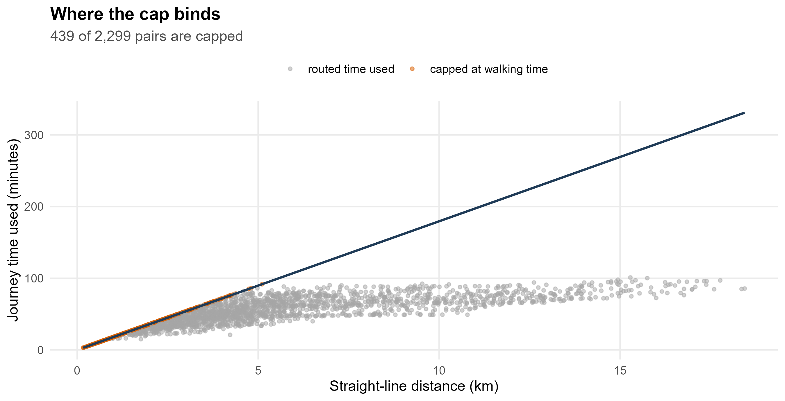
**Walking is always available.** Where the bus network is awkward the
router returns a poor itinerary: about a fifth of pairs came back slower
than simply walking the distance, in one case 99 minutes for 4 km. That
is a property of the router, not of the city, so every journey is capped
at the time it would take to walk:
$$c_{ij} \;=\; \min\!\left(c^{\text{routed}}_{ij},\;
\frac{d_{ij} \times `r sprintf("%.1f", acc$walk_fallback$circuity)`}{`r sprintf("%.2f", acc$walk_fallback$kmh)` \text{ km/h}} \times 60\right)$$
The walking pace comes from a systematic review of active school travel:
children's mean walking trip is
`r fmt_n(acc$walk_fallback$review$dist_m)` m in
`r sprintf("%.1f", acc$walk_fallback$review$time_min)` minutes, or
`r sprintf("%.2f", acc$walk_fallback$kmh)` km/h, and the circuity factor
of `r sprintf("%.1f", acc$walk_fallback$circuity)` turns straight-line
distance into street distance. The cap binds on
`r fmt_pct(100 * mean(costs$walk_capped), 0)` of pairs. **It is a ceiling
on modelled time, not a claim that children walk that far** — the same
review finds they rarely walk beyond 1.8 km.
**A distance model fills the gaps.** Where the matrix has no routed value
at all, a fitted model of time on straight-line distance stands in. It
reaches `r fmt_pct(100 - 100 * mean(costs$routed), 1)` of pairs in the
city, so almost everything here is routed rather than predicted.
```{r fig-cij-walk}
#| fig-cap: "Every zone-school pair: routed journey time against straight-line distance. The line is the walking time the cap uses. Points above it are journeys the router made slower than walking, and they are pulled down onto the line."
#| fig-height: 4.6
wk <- costs %>% mutate(walk_min = km * acc$walk_fallback$circuity / acc$walk_fallback$kmh * 60)
ggplot(wk, aes(km, cij)) +
  geom_point(aes(colour = walk_capped), size = 1.1, alpha = 0.5) +
  geom_line(aes(km, walk_min), colour = "#1f3b57", linewidth = 0.9) +
  scale_colour_manual(values = c(`FALSE` = "grey65", `TRUE` = "#d95f02"),
                      labels = c(`FALSE` = "routed time used",
                                 `TRUE` = "capped at walking time"), name = NULL) +
  labs(x = "Straight-line distance (km)", y = "Journey time used (minutes)",
       title = "Where the cap binds",
       subtitle = sprintf("%s of %s pairs are capped",
                          fmt_n(sum(costs$walk_capped)), fmt_n(nrow(costs)))) +
  theme_bh() + theme(legend.position = "top")
```
## What a journey-time surface looks like
```{r fig-cij-longhill}
#| fig-cap: "Journey time to Longhill from every neighbourhood, at its current site and at the Elm Grove site. Both panels use the same scale, so they can be read against each other. The white dot is the school."
#| fig-height: 5
lh_now <- to_lsoa(costs, LH) %>% mutate(site = "Ovingdean (today)")
lh_elm <- to_lsoa(cost_elm, LH) %>% mutate(site = "Elm Grove")
lh_map <- lsoa_sf %>%
  inner_join(bind_rows(lh_now, lh_elm), by = c("lsoa21cd" = "lsoa")) %>%
  mutate(site = factor(site, c("Ovingdean (today)", "Elm Grove")))
pts <- bind_rows(
  sch_sf %>% filter(name == LH) %>% mutate(site = "Ovingdean (today)"),
  st_as_sf(data.frame(e = oi$elm_grove$easting, n = oi$elm_grove$northing),
           coords = c("e", "n"), crs = 27700) %>% st_transform(4326) %>%
    mutate(site = "Elm Grove")) %>%
  mutate(site = factor(site, levels(lh_map$site)))
ggplot() +
  geom_sf(data = lh_map, aes(fill = cij), colour = NA) +
  geom_sf(data = catch_sf, fill = NA, colour = "white", linewidth = 0.25) +
  geom_sf(data = pts, shape = 21, fill = "white", colour = "black", size = 3, stroke = 1.1) +
  facet_wrap(~ site) +
  scale_fill_viridis_c(option = "magma", direction = -1, name = "Minutes") +
  labs(title = "The same school, two sites",
       subtitle = "Walk-and-bus journey time from each neighbourhood, weekday morning") +
  theme_void(12) +
  theme(plot.title = element_text(face = "bold", colour = "#1f3b57"),
        plot.subtitle = element_text(colour = "grey35"),
        strip.text = element_text(face = "bold"))
```
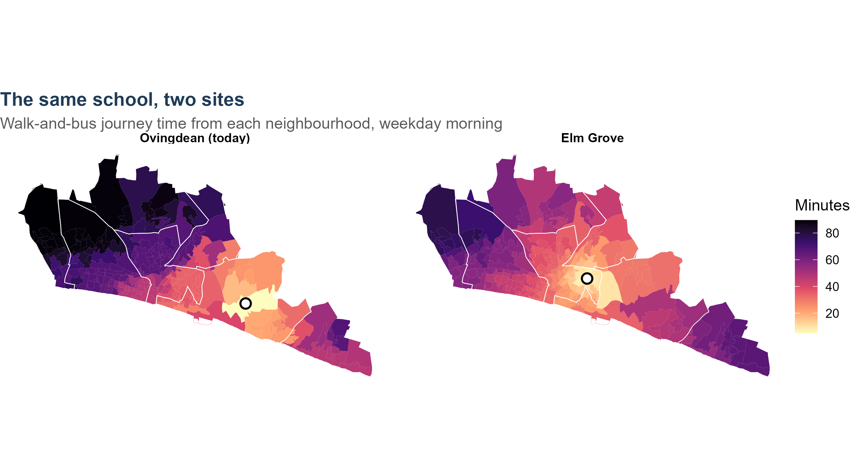
The median neighbourhood is
`r sprintf("%.0f", median(lh_now$cij))` minutes from Ovingdean and
`r sprintf("%.0f", median(lh_elm$cij))` from Elm Grove. That difference
is the whole of what relocation does to $c_{ij}$ — and, because nothing
else in the model moves with it except the competition term, most of what
relocation does at all.
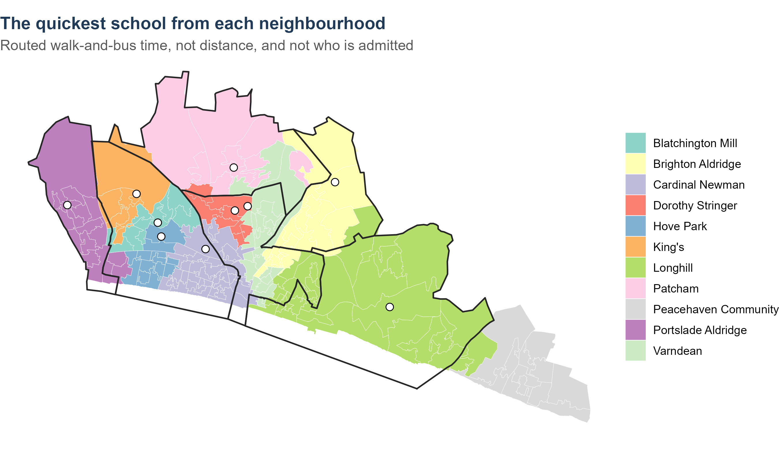
```{r fig-cij-nearest}
#| fig-cap: "Which school each neighbourhood can reach quickest, by routed walk-and-bus time. Boundaries are the catchments in force; where a colour crosses a boundary, the catchment school is not the nearest one."
#| fig-height: 5.2
nearest <- costs %>%
  inner_join(zone_lsoa, by = "zone") %>%
  group_by(lsoa, name) %>% summarise(cij = weighted.mean(cij, Oi), .groups = "drop_last") %>%
  slice_min(cij, n = 1, with_ties = FALSE) %>% ungroup() %>%
  mutate(School = short_sch(name))
near_map <- lsoa_sf %>% inner_join(nearest, by = c("lsoa21cd" = "lsoa"))
ggplot() +
  geom_sf(data = near_map, aes(fill = School), colour = "white", linewidth = 0.1) +
  geom_sf(data = catch_sf, fill = NA, colour = "grey15", linewidth = 0.6) +
  geom_sf(data = sch_sf, shape = 21, fill = "white", colour = "black", size = 2.6) +
  scale_fill_brewer(palette = "Set3", name = NULL) +
  labs(title = "The quickest school from each neighbourhood",
       subtitle = "Routed walk-and-bus time, not distance, and not who is admitted") +
  theme_void(12) +
  theme(plot.title = element_text(face = "bold", colour = "#1f3b57"),
        plot.subtitle = element_text(colour = "grey35"))
```
## A worked example
```{r cij-worked}
#| tbl-cap: "One neighbourhood's journey to every city school, with the straight-line distance beside it. The two are not the same ordering, which is the reason for routing at all."
ex_zone <- costs %>% filter(zone == ex_zones$zone[1])
ex_zone %>%
  arrange(cij) %>%
  transmute(School = short_sch(name), `Journey time (minutes)` = sprintf("%.0f", cij),
            `Straight line (km)` = sprintf("%.1f", km),
            Basis = ifelse(walk_capped, "capped at walking time",
                           ifelse(routed, "routed", "distance model"))) %>%
  knitr::kable(align = "lrrl")
```
### The same neighbourhood, routed {#sec-cij-routes}
```{r cij-routes-data}
#| include: false
gr <- bh_data("guide_routes.rds")
stopifnot(gr$origin$zone == ex_zones$zone[1])
# The four schools the text walks through come first in the switcher.
GR_FIRST <- c("Varndean School", "Brighton Aldridge Community Academy",
"Hove Park School", "King's School")
gr_sum <- gr$summary %>%
mutate(label = short_sch(school),
first = match(school, GR_FIRST)) %>%
arrange(is.na(first), first, model_minutes)
gr_legs <- gr$legs %>%
mutate(mode_lab = if_else(leg_mode == "WALK", "Walk", "Bus"),
label = short_sch(school))
# A label at the middle of every bus leg, carrying the service number.
mid_pt <- function(g) {
xy <- sf::st_coordinates(g)
xy[ceiling(nrow(xy) / 2), c("X", "Y")]
}
gr_bus <- gr_legs %>% filter(mode_lab == "Bus")
gr_bus_xy <- t(vapply(sf::st_geometry(gr_bus), mid_pt, numeric(2)))
gr_bus <- gr_bus %>% st_drop_geometry() %>%
mutate(lon = gr_bus_xy[, 1], lat = gr_bus_xy[, 2])
GR_COL <- c(Walk = "#e08214", Bus = "#2166ac")
gr_of <- function(s, col) gr_sum[[col]][gr_sum$label == s]
```
The table gives one number per school. Behind each number is a journey,
and it is worth seeing what the journey involves. The map routes the same
neighbourhood to every city school, leg by leg, on the same network and
the same weekday-morning timetable the model uses.
```{r fig-cij-routes}
#| fig-cap: "Indicative routes from the worked neighbourhood to each city school. Choose a school on the right. Walking legs are orange and follow the street network; bus legs are blue, follow the service's own route and are labelled with the service number. Schools the model caps at walking time are routed on foot only. The route starts at the neighbourhood's centre, so its time differs a little from the model's, which averages over every postcode in the neighbourhood. Both ends are snapped to the nearest street, so a line can stop just short of its marker."
gr_bb <- sf::st_bbox(gr_legs)
sch_pts <- schools_sf(oi$schools) %>%
  filter(name %in% gr_sum$school)

mr <- leaflet(width = "100%", height = 620) %>%
  add_basemap() %>%
  addPolygons(data = catch_sf, fill = FALSE, color = "#555555",
              weight = 1, opacity = 0.5, group = "Catchment boundaries")

for (i in seq_len(nrow(gr_sum))) {
  s <- gr_sum$school[i]; g <- gr_sum$label[i]
  d <- gr_legs %>% filter(school == s)
  b <- gr_bus %>% filter(school == s)
  leg_label <- function(x) sprintf("Leg %d: %s%s, %.0f min", x$leg, x$mode_lab,
                                   if_else(nzchar(x$route), paste0(" ", x$route), ""),
                                   x$minutes + x$wait)
  dw <- d %>% filter(mode_lab == "Walk")
  db <- d %>% filter(mode_lab == "Bus")
  if (nrow(dw))
    mr <- mr %>% addPolylines(data = dw, group = g, color = GR_COL[["Walk"]],
                              weight = 5, opacity = 0.9, dashArray = "6 6",
                              label = leg_label(dw))
  if (nrow(db))
    mr <- mr %>% addPolylines(data = db, group = g, color = GR_COL[["Bus"]],
                              weight = 5, opacity = 0.85, label = leg_label(db))
  mr <- mr %>%
    addCircleMarkers(data = sch_pts %>% filter(name == s), group = g,
                     radius = 7, color = "#111111", weight = 2, fillColor = "#ffffff",
                     fillOpacity = 1, label = ~ name) %>%
    addCircleMarkers(data = sch_pts %>% filter(name != s), group = g,
                     radius = 3, color = "#777777", weight = 1, fillColor = "#cccccc",
                     fillOpacity = 0.9, label = ~ name) %>%
    addCircleMarkers(lng = gr$origin$lon, lat = gr$origin$lat, group = g,
                     radius = 7, color = "#111111", weight = 2, fillColor = "#b2182b",
                     fillOpacity = 1, label = "The worked neighbourhood")
  if (nrow(b))
    mr <- mr %>%
      addLabelOnlyMarkers(lng = b$lon, lat = b$lat, group = g,
                          label = paste("Bus", b$route),
                          labelOptions = labelOptions(noHide = TRUE, direction = "top",
                                                      textOnly = FALSE,
                                                      style = list("font-weight" = "bold",
                                                                   "color" = "#2166ac")))
}

mr %>%
  fitBounds(lng1 = unname(gr_bb["xmin"]) - 0.005, lat1 = unname(gr_bb["ymin"]) - 0.004,
            lng2 = unname(gr_bb["xmax"]) + 0.005, lat2 = unname(gr_bb["ymax"]) + 0.004) %>%
  addLayersControl(baseGroups = gr_sum$label,
                   overlayGroups = "Catchment boundaries",
                   options = layersControlOptions(collapsed = FALSE)) %>%
  hideGroup("Catchment boundaries") %>%
  addLegend("bottomright", colors = unname(GR_COL), labels = names(GR_COL),
            title = "Leg", opacity = 0.9) %>%
  # Zoom to the chosen school's route, on load and whenever it changes.
  htmlwidgets::onRender("
    function(el, x) {
      var map = this;
      function fitRoute(group) {
        var b = L.latLngBounds([]);
        group.eachLayer(function(l) {
          if (l instanceof L.Polyline) b.extend(l.getBounds());
        });
        if (b.isValid()) map.fitBounds(b.pad(0.25), {maxZoom: 16});
      }
      map.on('baselayerchange', function(e) { fitRoute(e.layer); });
      setTimeout(function() {
        var active = el.querySelector('.leaflet-control-layers-base input:checked');
        if (!active || !active.nextSibling || !map.layerManager) return;
        var grp = map.layerManager.getLayerGroup(active.nextSibling.textContent.trim(), false);
        if (grp) fitRoute(grp);
      }, 300);
    }")
```
```{r cij-routes-table}
#| tbl-cap: "The routes on the map, against the model's journey time for the neighbourhood."
gr_sum %>%
  transmute(School = label,
            `Model (minutes)` = sprintf("%.0f", model_minutes),
            `This route (minutes)` = route_minutes,
            Legs = legs,
            `Buses, in order` = if_else(nzchar(services), gsub(" then ", " → ", services), "walk only"),
            Changes = changes,
            Basis = if_else(walk_capped, "walking", "walk and bus")) %>%
  knitr::kable(align = "lrrrlrl")
```
Four of them show the range:
- **Varndean** is a walk of about `r gr_of("Varndean", "route_minutes")`
minutes. The model caps it at walking time, because no bus journey
beats walking there.
- **Brighton Aldridge** is `r gr_of("Brighton Aldridge", "route_minutes")`
minutes by bus`r if (nzchar(gr_of("Brighton Aldridge", "services"))) paste0(" (", gsub(" then ", ", then ", gr_of("Brighton Aldridge", "services")), ")") else ""`,
with `r gr_of("Brighton Aldridge", "changes")` change.
- **Hove Park** is `r gr_of("Hove Park", "route_minutes")` minutes, with
`r gr_of("Hove Park", "changes")` changes, for a school
`r sprintf("%.1f", gr_of("Hove Park", "km"))` km away in a straight line.
- **King's** is `r gr_of("King's", "route_minutes")` minutes, with
`r gr_of("King's", "changes")` changes`r if (identical(gr_of("King's", "services"), gr_of("Hove Park", "services"))) ", on the same buses as Hove Park, carried further west" else ""`.
The ordering by time is not the ordering by distance, which is the
reason for routing at all. King's is
`r sprintf("%.1f", gr_of("King's", "km"))` km away and takes
`r gr_of("King's", "route_minutes")` minutes; Portslade Aldridge is
`r sprintf("%.1f", gr_of("Portslade Aldridge", "km"))` km away and takes
`r gr_of("Portslade Aldridge", "route_minutes")`, because
`r if (gr_of("Portslade Aldridge", "changes") < gr_of("King's", "changes")) "it needs one change fewer" else "its services line up better"`.
## The journeys the model does not route
- **The four schools outside the city** — Priory, Peacehaven, Seahaven
and Seaford Head — are chosen on **straight-line kilometres**, not
routed minutes. The bus network has no direct eastern service to Lewes,
so the routed journey from Woodingdean goes through Brighton and takes
over an hour, which is not what the families who make that journey do.
Their decay is fitted on km against the published 2024 destinations.
- **CoMArt**, when opened, is routed from its old site on the same
network and with the same parameters as every other school.
- **Longhill at Elm Grove** has a routed column of its own. An earlier
version had no routed times for the site and gave it the average
accessibility of a Brighton secondary, which was wrong by about sixty
children; the build now stops rather than let that happen silently.
## Corrected: Hove Park has two campuses {#sec-cij-hove-park}
```{r hp-campus}
#| include: false
hpv <- inp$hove_park_valley
HPN <- hpv$school
hp_km <- sqrt((inp$schools$easting[inp$schools$name == HPN] - hpv$easting)^2 +
(inp$schools$northing[inp$schools$name == HPN] - hpv$northing)^2) / 1000
hp_cost <- inp$cost$now %>%
filter(name == HPN) %>% select(zone, nevill = cij) %>%
inner_join(inp$cost$valley %>% filter(name == HPN) %>% select(zone, valley = cij),
by = "zone") %>%
mutate(d = valley - nevill)
hp_run <- function(hp, y = 2026)
run_sim(inp, year = y, rules = list(rule = "priorities"), hp_site = hp)
hp_v <- hp_run("valley"); hp_n <- hp_run("nevill")
hp_int <- function(r, s = HPN) r$schools$intake[r$schools$name == s]
# Where its children come from, by home ward. Ward names come with the
# council's own count (@sec-oi-ward-check).
hp_wards <- bh_data("ward_validation.rds")$counts %>% select(code = code, ward)
hp_wt <- oi$zones %>% group_by(zone) %>% mutate(w = Oi / sum(Oi)) %>% ungroup() %>%
select(zone, code = ward, w)
hp_by_ward <- function(r, lab) r$flows %>% filter(name == HPN) %>%
group_by(zone) %>% summarise(f = sum(flow), .groups = "drop") %>%
inner_join(hp_wt, by = "zone", relationship = "many-to-many") %>%
group_by(code) %>% summarise(!!lab := sum(f * w), .groups = "drop")
# The eastern outflow, for the note on the out-of-city fit below.
hp_priory <- hp_v$flows %>%
filter(name == "Priory School") %>%
group_by(zone) %>% summarise(f = sum(flow), .groups = "drop") %>%
inner_join(hp_wt, by = "zone", relationship = "many-to-many") %>%
group_by(code) %>% summarise(children = sum(f * w), .groups = "drop") %>%
inner_join(hp_wards, by = "code") %>% arrange(desc(children))
hp_comp <- hp_by_ward(hp_n, "nevill") %>%
inner_join(hp_by_ward(hp_v, "valley"), by = "code") %>%
inner_join(hp_wards, by = "code") %>%
mutate(change = valley - nevill) %>%
arrange(desc(abs(change)))
```
Every school in the cost table sits where the school register puts it,
which is the address the school gives. For Hove Park that address is the
Nevill Campus on Nevill Road. But Hove Park teaches **Years 7 and 8 at
the Valley Campus on Hangleton Way**, `r sprintf("%.2f", hp_km)` km
further west, and only moves pupils to Nevill Road in Year 9. This model
is about Year 7. Every journey time it used for Hove Park was therefore a
journey to a building the modelled children would not attend for two
years.
The error is not random. The Valley Campus is west of the Nevill Campus,
towards Hangleton and Portslade and away from central Hove and Brighton,
so putting Year 7 at Nevill Road makes the school look nearer than it is
to the parts of the city with most children in them, and further than it
is from Hangleton. Routed to both sites, the Valley Campus is a median
**`r sprintf("%+.1f", median(hp_cost$d))` minutes** from the city's
neighbourhoods, but quicker from the
`r sprintf("%.0f%%", 100 * mean(hp_cost$d < 0))` of them that lie west
and north west.
This is temporary. The council gave statutory notice on 8 June 2026 to
discontinue the Valley Campus on 31 August 2028 and consolidate the
school on Nevill Road from 1 September 2028. So the model now carries
both sites: **entry years up to 2027 are taught at Hangleton Way, 2028
onwards at Nevill Road**, and `run_sim()` picks the campus from the entry
year unless told otherwise. Everything fitted to preferences or offers —
attractiveness, the catchment terms, the competing-destinations term —
is fitted with Year 7 at the Valley Campus, because every round it is
fitted to was taught there.
```{r hp-campus-table}
#| tbl-cap: "The same entry year, run at each campus. Everything else is held: the same attractiveness, the same catchments, the same admission numbers."
tibble::tibble(
  Measure = c("Hove Park's intake",
              "Its mean journey",
              "Blatchington Mill's intake",
              "Portslade Aldridge's intake"),
  `Valley Campus` = c(
    sprintf("%.0f", hp_int(hp_v)),
    sprintf("%.1f min", hp_v$schools$mean_min[hp_v$schools$name == HPN]),
    sprintf("%.0f", hp_int(hp_v, "Blatchington Mill School")),
    sprintf("%.0f", hp_int(hp_v, "Portslade Aldridge Community Academy"))),
  `Nevill Road` = c(
    sprintf("%.0f", hp_int(hp_n)),
    sprintf("%.1f min", hp_n$schools$mean_min[hp_n$schools$name == HPN]),
    sprintf("%.0f", hp_int(hp_n, "Blatchington Mill School")),
    sprintf("%.0f", hp_int(hp_n, "Portslade Aldridge Community Academy")))) %>%
  knitr::kable(align = "lrr")
```
The totals barely move: `r sprintf("%.0f", abs(hp_int(hp_v) - hp_int(hp_n)))`
children on an intake of about `r sprintf("%.0f", hp_int(hp_v))`. That is
the answer to the obvious question, and it is worth stating plainly,
because it means the campus was **not** the reason the model has trouble
with Hove Park.
What does change, and changes a great deal, is **which children**:
```{r hp-campus-wards}
#| tbl-cap: "Hove Park's modelled Year 7, by home ward, at each campus. The six wards the campus matters most for."
hp_comp %>%
  slice_head(n = 6) %>%
  transmute(Ward = ward,
            `At the Valley Campus` = sprintf("%.0f", valley),
            `At Nevill Road` = sprintf("%.0f", nevill),
            Difference = sprintf("%+.0f", change)) %>%
  knitr::kable(align = "lrrr")
```
About a quarter of the school's intake changes ward. At Hangleton Way it
draws heavily on **Hangleton & Knoll**, the ward it actually sits in, and
on Portslade; at Nevill Road it draws instead on **Westdene & Hove Park**
and **Westbourne & Poets' Corner**. Those are different children, with
different journeys and a different level of disadvantage, so every
measure built on the composition of an intake — the segregation index,
deprived children's journey times, each school's free-school-meal share —
was being computed for the wrong families in the city's largest paired
catchment.
::: {.callout-note}
## What this does and does not fix
It does not fix Hove Park's intake. The model still puts more children
there than the school was offered in September 2026, and the reason lies
elsewhere: most of Hove Park's modelled intake is overflow refused at
Blatchington Mill, and the city's take-up of state places is not uniform
(@sec-oi-ward-check). Correcting the campus moves those children between
wards rather than out of the school.
What it fixes is the geography, which everything downstream is built on.
It also repaired a second fault it exposed: the out-of-city fit is a
likelihood with more than one basin, and moving Hove Park was enough to
send the optimiser into the wrong one, which cut the modelled flow from
Longhill's catchment to Priory School from about 35 children to almost
none, at a likelihood six times worse. The starting grid is wider now
and the fitted likelihood is reported, so the next time the geometry
moves this shows up rather than passing silently.
Two things say the recovered basin is the right one rather than merely
the better-fitting one. It reproduces the council's published 2024
destinations — 38 children from Longhill's catchment to Priory, against
35 modelled. And it puts them where local knowledge puts them: of the
`r sprintf("%.0f", sum(hp_priory$children))` children the model sends to
Priory, `r sprintf("%.0f%%", 100 * hp_priory$children[1] / sum(hp_priory$children))`
are from **`r hp_priory$ward[1]`**, the part of the city closest to
Lewes, and the next largest share is from
`r hp_priory$ward[2]`. That outflow is a real feature of the eastern edge of
the city and has no counterpart in the west, which is exactly why a
badly-fitted version of it is easy to miss: nothing on the Hove side of
the city would look wrong.
:::
## Checks you can run
```{r cij-checks}
#| tbl-cap: "What the cost table should satisfy, and what it gives."
st <- acc$statutory
tibble::tribble(
  ~Check, ~Result,
  "Every zone can reach every city school",
  sprintf("%s pairs, none missing", fmt_n(nrow(inp$cost$now))),
  "Journeys are routed rather than predicted",
  sprintf("%.1f%% routed", 100 * mean(costs$routed)),
  "No journey is slower than walking",
  sprintf("%.0f%% capped, none above the walk line", 100 * mean(costs$walk_capped)),
  "Mean journey to the catchment school",
  sprintf("%.1f minutes", st$mean_min),
  "Against the statutory limit for secondary (75 minutes)",
  sprintf("%.0f children over it", st$over_75_children),
  "Against the national average school journey (19 minutes)",
  sprintf("city mean %.1f minutes", st$mean_min)) %>%
  knitr::kable(align = "lr")
```
The strongest check is not in the table: a handful of journeys can be
compared against local knowledge. Woodingdean to Longhill comes out at
about 17 minutes and Woodingdean to Dorothy Stringer at about 68;
Whitehawk to Longhill about 28 and to Stringer about 62. Those are the
journeys that decide the eastern half of this work, and they are worth
checking against what a family there would say.
## What to be careful about
- **One departure, one day.** Every journey is a single weekday morning
in the timetable as it stood when the matrix was built. Term-time
variation, a missed connection and a cancelled bus are all outside it.
- **A mean over postcodes.** A zone's cost is the average of the
postcodes in it, so a neighbourhood with one badly connected corner
shows as slightly worse rather than showing both.
- **No cars, no lifts, no walking buses.** The model prices the journey a
child could make on foot and by bus. A family with a car makes a
different journey, and that is one reason the east's figures should be
read as a ceiling on difficulty rather than a description of it.
- **Time is symmetric here.** One morning journey stands for the return
as well, and no allowance is made for after-school travel.
- **The cap is generous at distance.** A 6 km walk is not a real school
journey, but capping at walking time is deliberately crude: it removes
router artefacts without inventing a bus that does not run.
## Questions this raises
1. Should the zone cost be the mean over its postcodes, or the
child-weighted mean, or the best available journey rather than the
average one?
2. Should journeys be routed at more than one departure time, so that a
thin early timetable is visible?
3. Should the out-of-city schools be routed rather than measured on
straight-line distance, if a feed covering East Sussex services were
used?
# $\beta$: how sharply distance deters {#sec-beta}
```{r beta-setup}
#| include: false
env <- bh_data("sensitivity_envelope.rds")
BETA <- inp$params$beta
ext <- cal$outside
```
## What it is
$\beta$ is the exponent on journey time. It converts the minutes of §4
into a pull:
$$\text{pull of school } j \text{ on neighbourhood } i \;\propto\; c_{ij}^{-\beta}$$
A larger $\beta$ means families discount distance more sharply. It is a
single number for the whole city, fixed at **`r sprintf("%.1f", BETA)`**,
and it is the same in every run of the simulator: no slider moves it.
The form matters as much as the value. This is a **power** decay, not an
exponential one: doubling the journey divides the pull by
$2^{`r sprintf("%.1f", BETA)`} \approx `r sprintf("%.1f", 2^BETA)`$,
whatever the starting point. That is the standard form in spatial
interaction modelling, and it behaves sensibly over the range of journeys
a city this size contains.
```{r fig-beta-curve}
#| fig-cap: "What the exponent does. Each curve is the pull of a school against journey time, scaled to 1 at ten minutes. The model uses 1.7; the sweep in the open model runs from 1.5 to 3.2."
#| fig-height: 4.4
bs <- c(1.5, BETA, 2.4, 3.2)
tidyr::expand_grid(beta = bs, mins = seq(10, 70, by = 0.5)) %>%
  mutate(pull = (mins^-beta) / (10^-beta),
         lab = sprintf("β = %.1f", beta),
         model = beta == BETA) %>%
  ggplot(aes(mins, pull, colour = lab, linewidth = model)) +
  geom_line() +
  scale_linewidth_manual(values = c(`FALSE` = 0.7, `TRUE` = 1.6), guide = "none") +
  scale_colour_manual(values = c("grey70", "#1f3b57", "grey55", "grey40"), name = NULL) +
  scale_y_continuous(labels = label_percent()) +
  labs(x = "Journey time (minutes)", y = "Pull, relative to a ten-minute journey",
       title = "A school twice as far away is a fraction as likely to be chosen",
       subtitle = sprintf("At β = %.1f, a 20-minute journey has %.0f%% of the pull of a 10-minute one, and 40 minutes has %.0f%%",
                          BETA, 100 * 2^-BETA, 100 * 4^-BETA)) +
  theme_bh() + theme(legend.position = "top")
```
## Where the value comes from, and what it is not
**It is a judgement, not an estimate.** Fitting $\beta$ properly needs
observed flows — how many children actually travel from each
neighbourhood to each school — and the council has not released them. A
catchment-level preference table identifies the catchment terms (§6, to
follow) but not distance decay, because within a catchment every family
is at a different distance and the table does not say who is where.
So `r sprintf("%.1f", BETA)` is a central value chosen for a system of
this kind: journeys are short, the alternatives sit close together, and
it is squarely inside the range this literature reports for school
choice. The open model does not rely on it being right. It runs
everything across `r length(env$betas)` values from
`r sprintf("%.1f", min(env$betas))` to `r sprintf("%.1f", max(env$betas))`
and reports which conclusions survive the whole range.
::: {.callout-note appearance="simple"}
## What would pin it down
A Poisson regression of flows on log journey time with an origin fixed
effect returns $\beta$ with a standard error, from records the admissions
process already produces. It is half a day's work on data the council
holds. Every band in the open model that comes from sweeping $\beta$
would become a number with an interval around it.
:::
## How much rests on it
```{r beta-importance}
#| tbl-cap: "What the open model's answer is actually sensitive to. Share of the variation in Longhill's modelled recruitment across the full sweep, by input."
env$importance %>%
  filter(term != "Residuals") %>%
  mutate(Input = recode(term,
    "w_spec" = "Which attractiveness specification",
    "factor(entry_year)" = "Which entry year",
    "site_label" = "Longhill's site",
    "factor(beta)" = "Distance decay (β)",
    "factor(gamma)" = "Strength of the catchment term (γ)")) %>%
  arrange(desc(pct)) %>%
  transmute(Input, `Share of the variation` = sprintf("%.1f%%", pct)) %>%
  knitr::kable(align = "lr")
```
**Distance decay is not the big unknown.** It accounts for
`r sprintf("%.0f%%", env$importance$pct[env$importance$term == "factor(beta)"])`
of the variation in the answer, against
`r sprintf("%.0f%%", env$importance$pct[env$importance$term == "w_spec"])`
for how attractive each school is taken to be. That is worth knowing
because it says what data would be worth having: school-level revealed
preference, more than travel behaviour.
```{r fig-beta-sweep}
#| fig-cap: "Longhill's modelled recruitment across the swept range of distance decay, at each attractiveness specification, 2026. The vertical line is the value the model uses. The spread between the coloured lines is the attractiveness question; the slope along each line is the distance-decay question."
#| fig-height: 4.8
env$envelope %>%
  filter(entry_year == 2026, gamma == 1.6) %>%
  mutate(site = ifelse(site == "now", "Ovingdean (today)", "Elm Grove")) %>%
  ggplot(aes(beta, natural_intake, colour = w_label, group = w_label)) +
  geom_vline(xintercept = BETA, colour = "grey45", linetype = "31") +
  geom_line(linewidth = 0.9) +
  facet_wrap(~ site) +
  scale_colour_brewer(palette = "Dark2", name = NULL) +
  expand_limits(y = 0) +
  labs(x = "Distance decay (β)", y = "Children recruited",
       title = "The slope along each line is what β decides",
       subtitle = "Longhill's recruitment with its own admission number unbinding, catchment term at 1.6") +
  theme_bh() + theme(legend.position = "top")
```
## What it looks like from one neighbourhood
```{r fig-beta-shares}
#| fig-cap: "One neighbourhood's children, shared between schools by journey time alone, at three values of the exponent. Attractiveness, catchment and capacity are all switched off here, so the only thing acting is distance."
#| fig-height: 4.6
zex <- costs %>% filter(zone == ex_zones$zone[1])
tidyr::expand_grid(beta = c(1.5, BETA, 3.2), zex) %>%
  group_by(beta) %>%
  mutate(share = cij^-beta / sum(cij^-beta),
         School = short_sch(name)) %>%
  ungroup() %>%
  mutate(lab = sprintf("β = %.1f", beta),
         School = forcats::fct_reorder(School, cij)) %>%
  ggplot(aes(share, School, fill = lab)) +
  geom_col(position = position_dodge(width = 0.75), width = 0.7) +
  scale_x_continuous(labels = label_percent()) +
  scale_fill_manual(values = c("grey72", "#1f3b57", "grey45"), name = NULL) +
  labs(x = "Share of the neighbourhood's children", y = NULL,
       title = sprintf("Distance alone, from %s", sub("[|].*$", "", ex_zones$zone[1])),
       subtitle = "Schools ordered by journey time. A steeper decay concentrates children on the nearest schools.") +
  theme_bh() + theme(legend.position = "top")
```
That is the whole of what the exponent does: at
`r sprintf("%.1f", 1.5)` the nearest school takes
`r sprintf("%.0f%%", 100 * with(zex, (cij^-1.5 / sum(cij^-1.5))[which.min(cij)]))`
of this neighbourhood's children on distance alone; at
`r sprintf("%.1f", 3.2)`, `r sprintf("%.0f%%", 100 * with(zex, (cij^-3.2 / sum(cij^-3.2))[which.min(cij)]))`.
## A second decay, on a different scale
The four schools outside the city do not use $\beta$ at all. They are
chosen on straight-line kilometres with a decay of their own, fitted to
the published 2024 destinations:
$$\text{pull of an out-of-city school} \;=\; W^{\text{ext}}_j \; d_{ij}^{-`r sprintf("%.1f", ext$decay)`}$$
`r sprintf("%.1f", ext$decay)` is far steeper than
`r sprintf("%.1f", BETA)`, and the two are not comparable: this one is on
kilometres rather than minutes, and it is doing a different job. It is
absorbing everything that stops a Brighton family choosing a school in
another authority — the admissions arrangements of a different council,
the absence of a school bus, the sheer unfamiliarity — and compressing it
into the one dimension the fit has. It reproduces the published pattern,
which is a low bar for four schools and one year of data, and it should
not be read as a behavioural estimate at all.
## Checks you can run
```{r beta-checks}
#| tbl-cap: "What the decay should produce, and what it gives at the value the model uses."
r_now <- run_sim(inp, year = 2026, rules = list(rule = "priorities"))
m_now <- outcomes(inp, r_now)
tibble::tribble(
  ~Check, ~Result,
  "The exponent the model runs at",
  sprintf("%.1f, unchanged in every scenario", BETA),
  "Mean modelled journey to the school a child attends",
  sprintf("%.1f minutes", m_now$mean_min),
  "Against the national average school journey",
  sprintf("%.0f minutes (National Travel Survey)", acc$benchmarks$nts_min),
  "Share of children modelled at a school in their own catchment",
  sprintf("%.0f%%", 100 * r_now$in_catch_share),
  "Sensitivity of the answer to the exponent",
  sprintf("%.0f%% of the variation in the sweep", env$importance$pct[env$importance$term == "factor(beta)"])) %>%
  knitr::kable(align = "lr")
```
The mean modelled journey sits above the national average, which is what
a city with a coastal edge and one school in the far east should produce.
If it came out at or below the national figure, either the decay or the
journey times would be wrong.
## What to be careful about
- **One exponent for the whole city.** Families differ in how far they
will travel, and the literature is consistent that the willingness
varies with income and with whether a car is available. A single
$\beta$ averages over that, and it is the assumption most likely to
matter for the equity questions in the strategic view.
- **Everything else is fitted *given* this value.** The attractiveness
balancing (§3) and the catchment terms (§6) are estimated with $\beta$
held at `r sprintf("%.1f", BETA)`. A different decay would give
different fitted values for both, which is why the sweep re-runs the
whole model rather than swapping the exponent at the end.
- **Time, not distance, and not cost.** A journey that is quick but
requires two buses and a fare is treated as a short journey.
- **The floor at short journeys.** A power decay rises steeply as time
approaches zero, so the very shortest journeys carry a lot of weight.
The routed minimum in the table is
`r sprintf("%.0f", min(costs$cij))` minutes, which keeps it in bounds.
## Questions this raises
1. Should $\beta$ vary between groups of families — by deprivation, or by
whether a catchment has one school or two — rather than being one
number for the city?
2. Is the power form right, or would an exponential decay fit the pattern
of Brighton's journeys better? Both are standard; they differ most at
the long-journey end, which is where the eastern questions sit.
3. Should the out-of-city decay be re-fitted once more than one year of
destination data is available, or replaced by a proper choice model
for schools in another authority?
# $\gamma_h$: how much living in the catchment counts {#sec-gamma}
```{r gamma-setup}
#| include: false
gam <- cal$gamma
gam_lab <- setNames(unname(CATCH_LABELS[CATCH_FROM_MODEL[names(gam)]]), names(gam))
r_now <- run_sim(inp, year = 2026, rules = list(rule = "priorities"))
```
## What it is
$\gamma_h$ is the bonus a school gets for being **in the family's own
catchment**. It sits in the exponent, so it multiplies a school's pull:
$$\text{pull} \;\propto\; W_j\, c_{ij}^{-\beta} \times
\begin{cases} e^{\gamma_{h(i)}} & \text{if } j \text{ is a school of } i\text{'s catchment}\\ 1 & \text{otherwise}\end{cases}$$
The subscript matters: $\gamma$ is indexed by **$h(i)$, the catchment the
family lives in**, not by the school. Stringer / Varndean families are
modelled as following their map more closely than Brighton Aldridge's
families follow theirs, and that is a statement about families rather
than about schools.
::: {.callout-important}
## This is about what families name, not about who gets admitted
Admission priority is a separate stage of the model (§9):
when a school is oversubscribed the council's criteria decide who is
offered a place, and living in the catchment is one of them. $\gamma_h$
is doing something different and earlier. It says how much more likely a
family is to **want** a school because it is the one their map points
them to — through habit, siblings, the school bus, or simply reading the
catchment as a statement about where their child belongs.
The distinction is why the strategic view can find that catchment
priority allocates nothing at an undersubscribed school while the
catchment still matters a great deal there: nobody is turned away, but
the map still shapes what families ask for.
:::
## The fitted values
```{r gamma-table}
#| tbl-cap: "The catchment term fitted for each catchment, and what it does to a school's pull. A term of 0 would mean the map makes no difference to what families name."
tibble(catchment = names(gam), gamma = as.numeric(gam)) %>%
  mutate(Catchment = unname(gam_lab[catchment]),
         `Fitted $\\gamma_h$` = sprintf("%.1f", gamma),
         `Multiplies a catchment school's pull by` = sprintf("%.1f×", exp(gamma))) %>%
  arrange(desc(gamma)) %>%
  select(Catchment, `Fitted $\\gamma_h$`, `Multiplies a catchment school's pull by`) %>%
  knitr::kable(align = "lrr")
```
```{r fig-gamma-map}
#| fig-cap: "The fitted catchment term by catchment. Darker is a population that follows its map more closely, once distance and attractiveness are accounted for."
#| fig-height: 5
gsf <- catch_sf %>%
  left_join(tibble(catchment = unname(CATCH_FROM_MODEL[names(gam)]),
                   gamma = as.numeric(gam)), by = "catchment")
ggplot() +
  geom_sf(data = gsf, aes(fill = gamma), colour = "white", linewidth = 0.5) +
  geom_sf(data = sch_sf, shape = 21, fill = "white", colour = "black", size = 2.6) +
  geom_sf_text(data = gsf %>% st_point_on_surface() %>% suppressWarnings(),
               aes(label = sprintf("%.1f", gamma)), size = 5, fontface = "bold",
               colour = "white", nudge_y = 0.006) +
  scale_fill_viridis_c(option = "mako", direction = -1, name = "γ") +
  coord_sf(expand = TRUE) +
  labs(title = "How closely each catchment's families follow their map",
       subtitle = "Fitted to the council's catchment-level preference table") +
  theme_void(12) +
  theme(plot.title = element_text(face = "bold", colour = "#1f3b57"),
        plot.subtitle = element_text(colour = "grey35"))
```
Stringer / Varndean, at `r sprintf("%.1f", gam[["DS_Varndean"]])`, and
Longhill, at `r sprintf("%.1f", gam[["Longhill"]])`, are the two most
attached populations in the city; Brighton Aldridge's, at
`r sprintf("%.1f", gam[["BACA"]])`, the least. Those two facts do much of
the work in every relocation and redraw result in the strategic view,
because a move trades one against the other.
## How they are fitted
The council's evidence to the Schools Adjudicator includes a
catchment-level preference table: how many first, second and third
preferences each catchment's children gave each school, pooled over
`r length(mt$calibrated$rounds)` rounds. That is a flow matrix — coarse,
but a matrix — and it is enough to fit one term per catchment.
The loop is:
1. Take the current catchment terms and **balance $W_j$** so the model
reproduces each school's share of the city's first preferences (§3).
2. For one catchment, try every $\gamma$ on a grid from
`r sprintf("%.0f", 0)` to `r sprintf("%.0f", 4)` in steps of 0.1,
re-balancing $W_j$ at each step, and keep the value that minimises the
**Poisson deviance** between the modelled and observed shares in that
table.
3. Repeat for each catchment, then sweep again until nothing moves.
The deviance is the right loss here because the cells are counts of
preferences: it weights a cell by how many families it contains, so a
catchment that gives 400 first preferences counts for more than one that
gives 40.
```{r fig-gamma-profile}
#| fig-cap: "The fit against each candidate value, catchment by catchment. The point is the value chosen: the bottom of each curve. A flat curve would mean the data cannot distinguish one value from another."
#| fig-height: 5
cal$profile %>%
  mutate(Catchment = unname(gam_lab[catchment])) %>%
  group_by(Catchment) %>%
  mutate(rel = deviance - min(deviance)) %>%
  ungroup() %>%
  ggplot(aes(gamma, rel)) +
  geom_line(colour = "#1f3b57", linewidth = 0.9) +
  geom_point(data = ~ .x %>% group_by(Catchment) %>% slice_min(rel, n = 1),
             colour = "#d95f02", size = 2.6) +
  facet_wrap(~ Catchment, scales = "free_y") +
  labs(x = "Catchment term (γ)", y = "Deviance above the best fit",
       title = "Each catchment's own curve, and where it bottoms out",
       subtitle = "Lower is a better fit to the council's preference table") +
  theme_bh(11)
```
## What the fitting buys
```{r gamma-fit}
#| tbl-cap: "How well each specification reproduces the council's preference table. M4 is one catchment term for the whole city, fitted against offers; M5 is one per catchment, fitted against preferences."
cal$fit %>%
  transmute(Model = ifelse(model == "M4", "One term for the whole city (M4)",
                           "One term per catchment (M5)"),
            `Poisson deviance` = fmt_n(deviance),
            `Cell error (percentage points)` = sprintf("%.1f", cell_rmse_pp)) %>%
  knitr::kable(align = "lrr")
```
```{r fig-gamma-own}
#| fig-cap: "The share of each catchment's first preferences that go to its own school or schools: what the council's table records, and what each specification produces."
#| fig-height: 4.6
cal$own %>%
  mutate(Catchment = unname(gam_lab[home])) %>%
  tidyr::pivot_longer(c(observed, M4, M5), names_to = "src", values_to = "share") %>%
  mutate(src = recode(src, observed = "Observed",
                      M4 = "One term for the city", M5 = "One term per catchment"),
         src = factor(src, c("Observed", "One term for the city", "One term per catchment")),
         Catchment = forcats::fct_reorder(Catchment, share, .fun = max)) %>%
  ggplot(aes(share, Catchment, colour = src, shape = src)) +
  geom_point(size = 3.6) +
  scale_colour_manual(values = c("#1f3b57", "grey65", "#d95f02"), name = NULL) +
  scale_shape_manual(values = c(16, 15, 17), name = NULL) +
  scale_x_continuous(labels = label_percent()) +
  labs(x = "Share of the catchment's first preferences going to its own school", y = NULL,
       title = "A single city-wide term cannot reproduce the pattern",
       subtitle = "Fitting one term per catchment does, and it is the same model otherwise") +
  theme_bh() + theme(legend.position = "top")
```
The gain is large and it is concentrated where it matters. A single
city-wide term puts Stringer / Varndean's own-school share at
`r fmt_pct(100 * cal$own$M4[cal$own$home == "DS_Varndean"], 0)` against an
observed `r fmt_pct(100 * cal$own$observed[cal$own$home == "DS_Varndean"], 0)`,
and Longhill's at
`r fmt_pct(100 * cal$own$M4[cal$own$home == "Longhill"], 0)` against
`r fmt_pct(100 * cal$own$observed[cal$own$home == "Longhill"], 0)`. Fitting
each catchment separately reproduces both.
## The two schools with no catchment at all {#sec-gamma-faith}
```{r gamma-faith}
#| include: false
catch_lab <- function(x) {
out <- unname(CATCH_LABELS[CATCH_FROM_MODEL[x]])
dplyr::coalesce(out, x)
}
faith_n <- inp$schools$name[inp$schools$city & inp$schools$faith]
d_g <- r_now$flows
faith_rows <- d_g %>% filter(name %in% faith_n)
faith_mix <- d_g %>%
filter(name %in% c(faith_n, "Varndean School", "Longhill High School")) %>%
group_by(name, catchment) %>% summarise(n = sum(flow), .groups = "drop") %>%
group_by(name) %>% mutate(share = n / sum(n)) %>% ungroup()
faith_min <- d_g %>% group_by(name) %>%
summarise(min = weighted.mean(cij, flow), n = sum(flow), .groups = "drop")
city_min <- faith_min %>%
filter(name %in% inp$schools$name[inp$schools$city & !inp$schools$faith], n > 1)
faith_kern <- sum(inp$params$overflow[grepl(paste(faith_n, collapse = "|"),
names(inp$params$overflow))])
```
Cardinal Newman and King's are in **no catchment**, on any of the maps
the simulator carries. That is not a simplification: neither school has
one. Admission to Cardinal Newman turns on Catholic baptism and practice,
and King's is a Church of England free school with its own criteria and
no geographic area attached.
So $\gamma_h$ never applies to them. Every one of the
`r fmt_n(nrow(faith_rows))` neighbourhood-to-faith-school pairs in the
model has the indicator $\mathbb{1}[\,i \in \text{catchment}(j)\,]$ set to
zero, and their pull is $W_j\, c_{ij}^{-\beta}\, C_j^{\delta}$ and nothing
else. Four consequences follow, and they are worth being explicit about:
between them these two schools take
`r fmt_pct(100 * sum(faith_rows$flow) / sum(d_g$flow))` of the city's
Year 7 children.
**Their attractiveness carries the religion.** A family's faith is not in
this model — no published dataset gives it by neighbourhood. What the
fitting sees is that a great many families across the whole city name
these schools first anyway, and the only term free to explain it is
$W_j$. So Cardinal Newman ends up with the highest attractiveness in the
city (`r sprintf("%.2f", W5[["Cardinal Newman Catholic School"]])` against
a mean of 1) and King's the second
(`r sprintf("%.2f", W5[["King's School"]])`). Read those two numbers as
"wanted, city-wide, for reasons the model does not contain" rather than
as a judgement of the school.
**Distance is the only thing holding them in place.** With no catchment
bonus, $c_{ij}^{-\beta}$ is the sole spatial control on where their
children come from — which is why they draw from everywhere and why
their intakes travel furthest:
```{r fig-gamma-faith}
#| fig-cap: "Where each school's intake comes from, by the family's home catchment. The two faith schools have no catchment of their own, so nothing anchors them to one part of the city."
#| fig-height: 4.4
faith_mix %>%
  mutate(School = short_sch(name),
         School = factor(School, c("Cardinal Newman", "King's", "Varndean", "Longhill")),
         Catchment = catch_lab(catchment)) %>%
  ggplot(aes(share, forcats::fct_rev(School), fill = Catchment)) +
  geom_col(width = 0.7, colour = "white", linewidth = 0.4) +
  scale_x_continuous(labels = scales::percent) +
  scale_fill_brewer(palette = "Set2", name = "Home catchment") +
  labs(x = NULL, y = NULL,
       title = "Two schools drawn from the whole city, two from one corner of it",
       subtitle = "Modelled intake by the family's home catchment, 2026 entry") +
  theme_bh() + theme(legend.position = "right")
```
The children the model sends to King's travel
`r sprintf("%.0f", faith_min$min[faith_min$name == "King's School"])`
minutes on average and to Cardinal Newman
`r sprintf("%.0f", faith_min$min[faith_min$name == "Cardinal Newman Catholic School"])`,
against
`r sprintf("%.0f", min(city_min$min))` to
`r sprintf("%.0f", max(city_min$min))`
minutes at the eight community and academy schools. That is a real
feature of faith admissions, and the model reproduces it without being
told to.
**They are outside the catchment machinery everywhere else too.** The
priority-6 rule — a child from a single-school catchment applying outside
it — is defined on the catchment design, so it neither sends children to
these two nor gives them any standing there. When a boundary is redrawn
in a scenario, nothing about Cardinal Newman or King's changes except
through everyone else's movements. And because they are not community
schools, they are rationed by the proportional ceiling rather than by the
council's tiers (§9): the model has no representation of baptism
certificates or church attendance, so it treats an oversubscribed faith
school as a lottery over everyone who applied.
**They still take part in everything that is not the catchment.** They
compete in $C_j$ (§7) — Cardinal Newman is the second largest
contribution to Dorothy Stringer's competition term — they sit in every
neighbourhood's choice set and denominator (§8), and families do name
them as second preferences, so refused children are re-offered places
there: `r fmt_pct(100 * faith_kern / 6)` of a catchment's second
preferences go to one of the two on average (§10).
::: {.callout-warning}
## What this means for a faith-school scenario
Because the religion is inside $W_j$ rather than in a term of its own,
the simulator cannot distinguish "Cardinal Newman becomes less
attractive" from "fewer families in the city are practising Catholics".
Both are the same slider. A scenario that changes either should be read
as changing the *total* pull of the school, and the model will
redistribute those children by distance and catchment like anyone
else's — which is almost certainly too smooth a picture of what a
change in faith admissions would actually do.
:::
## What the slider does
The simulator's catchment slider multiplies **every** fitted term by the
same factor, from 0 to 2. At 0 the map stops mattering to what families
name and the model becomes distance and attractiveness alone; at 2 every
catchment's attachment doubles in the exponent, which is a very strong
map indeed. At 1 it uses the fitted values.
That single multiplier is deliberately blunt. It answers "what if
families follow their catchments more, or less, than they do now?"
without pretending to know which catchment would change.
```{r gamma-slider}
#| tbl-cap: "What the slider does to the share of children modelled at a school in their own catchment, 2026, council priorities."
purrr::map_dfr(c(0, 0.5, 1, 1.5, 2), function(g) {
  rr <- run_sim(inp, year = 2026, gamma = g, rules = list(rule = "priorities"))
  tibble(`Slider` = sprintf("%.1f×", g),
         `At a school in their own catchment` = fmt_pct(100 * rr$in_catch_share, 0))
}) %>%
  knitr::kable(align = "lr")
```
## Where it sits in the matrix
Unlike $O_i$ and $W_j$, the catchment term does not live in a margin. It
is a **mask over the interior**: for each neighbourhood, the cells of
schools in its own catchment are multiplied by $e^{\gamma_h}$ and the
rest are left alone.
```{r matrix-gamma}
#| tbl-cap: "The four neighbourhoods again. A cell marked with the multiplier is one where the school is in that neighbourhood's catchment; the others are untouched."
dsg <- inp$designs[["Current catchments"]]
cellmark <- function(zone, school) {
  in_c <- !is.na(dsg$school[school]) && dsg$school[school] == dsg$zone[zone]
  h <- unname(dsg$zone[zone])
  if (in_c) sprintf("$T_{ij} \\times %.1f$", exp(gam[[h]])) else "$T_{ij}$"
}
data.frame(
  Neighbourhood = c(sub("[|].*$", "", ex_zones$zone), "$W_j$"),
  `Dorothy Stringer` = c(vapply(ex_zones$zone, cellmark, "", school = sch4[1]),
                         sprintf("%.2f", W5[[sch4[1]]])),
  Varndean = c(vapply(ex_zones$zone, cellmark, "", school = sch4[2]),
               sprintf("%.2f", W5[[sch4[2]]])),
  Longhill = c(vapply(ex_zones$zone, cellmark, "", school = sch4[3]),
               sprintf("%.2f", W5[[sch4[3]]])),
  `Cardinal Newman` = c(vapply(ex_zones$zone, cellmark, "", school = sch4[4]),
                        sprintf("%.2f", W5[[sch4[4]]])),
  `$O_i$ (2026)` = c(sprintf("%.1f", ex_zones$Oi), ""),
  check.names = FALSE) %>%
  knitr::kable(align = "lccccr")
```
Cardinal Newman is in nobody's catchment: it and King's admit city-wide
on faith criteria, so no cell in their columns is ever multiplied. In the
two paired catchments **both** schools are in catchment, which is what
makes those catchments different objects from the four single-school
ones.
## Checks you can run
```{r gamma-checks}
#| tbl-cap: "What the catchment terms should satisfy."
prof_flat <- cal$profile %>% group_by(catchment) %>%
  summarise(span = diff(range(deviance)), .groups = "drop")
tibble::tribble(
  ~Check, ~Result,
  "Every catchment's fit has an interior minimum",
  sprintf("fitted %.1f to %.1f, grid 0 to 4", min(gam), max(gam)),
  "The data can tell one value from another",
  sprintf("deviance spans %s to %s across the grid",
          fmt_n(min(prof_flat$span)), fmt_n(max(prof_flat$span))),
  "Fitting per catchment beats one term for the city",
  sprintf("deviance %s against %s", fmt_n(cal$fit$deviance[cal$fit$model == "M5"]),
          fmt_n(cal$fit$deviance[cal$fit$model == "M4"])),
  "Modelled children at a catchment school, today",
  fmt_pct(100 * r_now$in_catch_share, 0),
  "Slider at zero removes the map entirely",
  fmt_pct(100 * run_sim(inp, year = 2026, gamma = 0,
                        rules = list(rule = "priorities"))$in_catch_share, 0)) %>%
  knitr::kable(align = "lr")
```
## What to be careful about
::: {.callout-warning}
## The assumption every redraw result depends on
The terms are fitted on the map families have lived with, and then
**carried unchanged to any other map**. A redraw in the simulator moves
which schools count as in catchment; it does not change how strongly a
family follows the line.
That is the single most consequential assumption in this work. If
families follow a new boundary less closely than the one they know —
which the strategic view finds some evidence for in what happened after
2024 — then every redraw result here is too optimistic about how many
children the redraw moves. The strategic view reports the halved-term
version of the relocation runs for exactly this reason.
:::
- **The term is fitted on the pre-2024 map**, because that is the map the
preference table covers.
- **It bundles several mechanisms.** Siblings already at the school, the
free bus, habit, and the sense that the catchment school is *the*
school all end up in one number, because the table cannot separate
them.
- **It is a home-catchment term, not a school term.** A school in two
catchments — none exist today, but CoMArt opening would create one —
takes each catchment's own strength.
- **Paired catchments are a single object here.** A Stringer / Varndean
family gets the bonus on both schools, and which of the two they prefer
is left to $W_j$, distance, and the exclusivity populations.
## Questions this raises
1. Should the term decay when a boundary changes — a family newly placed
in a catchment following it less closely than one that has been in it
for years?
2. Should it vary with how many schools a catchment contains, rather than
being one number per catchment?
3. Would first preferences by small area, before and after the 2024
change, let the normative half of this be separated from the
procedural half?
# $C_j$ and $\delta$: the company a school keeps {#sec-cj}
```{r cj-setup}
#| include: false
DELTA <- inp$params$delta
SIGMA <- inp$params$sigma
sch_city <- inp$schools[inp$schools$city & !(inp$schools$hypothetical %in% TRUE), ]
W_run <- setNames(sch_city$W, sch_city$name)
xy <- sch_city %>% select(name, easting, northing)
pairs_km <- tidyr::expand_grid(name = xy$name, k = xy$name) %>%
filter(name != k) %>%
left_join(xy, by = "name") %>%
left_join(xy %>% rename(k = name, ke = easting, kn = northing), by = "k") %>%
mutate(km = pmax(sqrt((easting - ke)^2 + (northing - kn)^2) / 1000, 0.1),
Wk = unname(W_run[k]), contrib = Wk * km^-SIGMA,
short = short_sch(name), k_short = short_sch(k))
sch_elm <- sch_city
lh_row <- sch_elm$name == "Longhill High School"
sch_elm$easting[lh_row] <- sch_city$elm_easting[lh_row]
sch_elm$northing[lh_row] <- sch_city$elm_northing[lh_row]
C_now <- compete_now(sch_city, W_run, SIGMA)
C_elm <- compete_now(sch_elm, W_run, SIGMA)
Cj <- tibble(name = names(C_now), C = unname(C_now),
C_elm = unname(C_elm[names(C_now)])) %>%
mutate(short = short_sch(name), index = 100 * C / mean(C),
index_elm = 100 * C_elm / mean(C), mult = (C / mean(C))^DELTA)
cj_of <- function(s, col) Cj[[col]][Cj$short == s]
min_km <- function(s) min(pairs_km$km[pairs_km$short == s])
rmse0 <- function(x) x$rmse[abs(x$value) < 1e-8]
r2_0 <- function(x) x$r2[abs(x$value) < 1e-8]
```
## What it is
$C_j$ measures **how much company a school has**: how many other schools
stand close to it, weighted by how wanted each of them is.
$$C_j \;=\; \sum_{k \neq j} W_k\, d_{jk}^{-\sigma}, \qquad \sigma = `r sprintf("%.0f", SIGMA)`$$
$d_{jk}$ is the straight-line distance in kilometres between two
**schools**, and it deliberately carries a different symbol from
$c_{ij}$: nobody travels from one school to another, so routing it would
mean nothing. All that is wanted is a measure of how clustered the
schools are. With $\sigma$ at `r sprintf("%.0f", SIGMA)` the term reduces
to *the sum of the rivals' attractiveness per kilometre they are away*.
It enters the model as a power on the pull:
$$\text{pull} \;\propto\; W_j\, c_{ij}^{-\beta}\, e^{\gamma_{h}\mathbb{1}[\cdot]}\, C_j^{\,\delta}, \qquad \delta = `r sprintf("%+.1f", DELTA)`$$
The reasoning is Fotheringham's: a plain gravity model is misspecified
when destinations cluster, because people choose an area first and a
destination within it second. Left out, the clustering does not go away —
it is absorbed by the distance parameter instead.
## Brighton in one term
```{r fig-cj-map}
#| fig-cap: "Each school sized by the company it keeps, with its score on an index where the city average is 100. The lines open up the two extremes: every rival's contribution to Dorothy Stringer's total in orange, and to Longhill's in navy. A thicker line is a bigger contribution."
#| fig-height: 5.0
sch_pts <- sch_city %>%
  select(name, easting, northing) %>%
  st_as_sf(coords = c("easting", "northing"), crs = 27700) %>%
  st_transform(4326) %>%
  mutate(short = short_sch(name),
         lon = st_coordinates(.)[, 1], lat = st_coordinates(.)[, 2]) %>%
  left_join(Cj %>% select(name, C, index), by = "name")
lonlat <- sch_pts %>% st_drop_geometry() %>% select(name, lon, lat)
segs <- pairs_km %>%
  filter(short %in% c("Dorothy Stringer", "Longhill")) %>%
  left_join(lonlat, by = "name") %>%
  left_join(lonlat %>% rename(k = name, klon = lon, klat = lat), by = "k")

ggplot() +
  geom_sf(data = catch_sf, fill = "grey96", colour = "white", linewidth = 0.5) +
  geom_segment(data = segs, aes(x = lon, y = lat, xend = klon, yend = klat,
                                linewidth = contrib, colour = short), alpha = 0.5) +
  geom_sf(data = sch_pts, aes(size = C), shape = 21, fill = "white",
          colour = "black", stroke = 0.9) +
  ggrepel::geom_text_repel(
    data = sch_pts, aes(lon, lat, label = sprintf("%s\n%.0f", short, index)),
    size = 2.9, lineheight = 0.9, colour = "#1f3b57", seed = 11,
    box.padding = 0.45, point.padding = 0.3, min.segment.length = 0.2,
    segment.colour = "grey55", segment.size = 0.3, max.overlaps = Inf) +
  scale_linewidth_continuous(range = c(0.2, 3.4), guide = "none") +
  scale_size_continuous(range = c(2, 9), guide = "none") +
  scale_colour_manual(values = c(`Dorothy Stringer` = "#d95f02", Longhill = "#1f3b57"),
                      name = NULL,
                      labels = function(x) paste("contributions to", x)) +
  coord_sf(expand = TRUE, clip = "off") +
  labs(title = "Five hundred metres from a rival, or five kilometres",
       subtitle = "The competing-destinations term by school, city average = 100") +
  theme_void(12) +
  theme(plot.title = element_text(face = "bold", colour = "#1f3b57"),
        plot.subtitle = element_text(colour = "grey35"),
        legend.position = "top")
```
The two ends of the city are different objects on this measure.
```{r cj-contrib}
#| tbl-cap: "What the term is made of at its two extremes. Each row is one rival: how far away it is, how wanted it is, and what it therefore contributes."
pairs_km %>%
  filter(short %in% c("Dorothy Stringer", "Longhill")) %>%
  group_by(short) %>% arrange(desc(contrib), .by_group = TRUE) %>%
  mutate(rank = row_number(), total = sum(contrib)) %>%
  filter(rank <= 3) %>% ungroup() %>%
  transmute(School = sprintf("%s (total %.2f)", short, total),
            Rival = k_short, `Distance (km)` = sprintf("%.2f", km),
            `Its $W_k$` = sprintf("%.2f", Wk),
            Contribution = sprintf("%.2f", contrib)) %>%
  knitr::kable(align = "llrrr")
```
Varndean stands `r sprintf("%.0f", 1000 * min_km("Dorothy Stringer"))`
metres from Dorothy Stringer, and Cardinal Newman — the most wanted
school in the city on $W_j$ — is under two kilometres from both. Those
two rivals alone contribute more to Stringer's term than **all nine** of
Longhill's rivals contribute to its own. On an index with the city
average at 100, Stringer scores
`r sprintf("%.0f", cj_of("Dorothy Stringer", "index"))` and Longhill
`r sprintf("%.0f", cj_of("Longhill", "index"))`.
Two features of the term follow from how it is built, and both matter in
the simulator:
- **It uses the attractiveness in force, not a fixed table.** Pull an
attractiveness slider and every *other* school's $C_j$ moves too,
because $W_k$ sits inside the sum.
- **It is a sum over the schools that exist in a run.** Close a school and
its neighbours lose the company it was providing; open CoMArt in East
Brighton and Longhill gains some.
## What the fitted exponent does
$\delta$ was fitted by grid search over
`r sprintf("%+.1f to %+.1f", min(mt$delta_fit$value), max(mt$delta_fit$value))`,
against the offers the council made in the most recent round, with the
capacity ceiling and the catchment term already in place (§6 explains why
the ceiling goes in first).
```{r fig-cj-delta}
#| fig-cap: "How much the term improves the fit, for three versions of the model. Each curve is that version's error against the offers made, relative to itself at δ = 0, so below 1 means the term is earning its place. The shaded half is the sign Fotheringham's argument predicts."
#| fig-height: 4.8
dprof <- bind_rows(
  mt$delta_fit   %>% mutate(v = "With the ceiling and the catchment term"),
  mt$delta_alone %>% mutate(v = "With the ceiling only"),
  mt$delta_nocap %>% mutate(v = "With neither")) %>%
  group_by(v) %>% mutate(rel = rmse / rmse[abs(value) < 1e-8]) %>% ungroup() %>%
  mutate(v = factor(v, c("With the ceiling and the catchment term",
                         "With the ceiling only", "With neither")))
ggplot(dprof, aes(value, rel, colour = v)) +
  annotate("rect", xmin = min(dprof$value), xmax = 0, ymin = -Inf, ymax = Inf,
           fill = "#b2182b", alpha = 0.05) +
  geom_hline(yintercept = 1, colour = "grey60", linewidth = 0.4) +
  geom_line(linewidth = 1) +
  geom_point(data = dprof %>% group_by(v) %>% slice_min(rel, n = 1) %>% ungroup(),
             size = 3, show.legend = FALSE) +
  annotate("text", x = min(dprof$value) + 0.05, y = 1.55, hjust = 0, vjust = 1,
           size = 3.5, colour = "#b2182b", lineheight = 0.95,
           label = "rivals take share\n(competing destinations)") +
  scale_colour_manual(values = c("#1f3b57", "#d95f02", "grey60"), name = NULL) +
  coord_cartesian(ylim = c(0.8, 1.6)) +
  labs(x = "δ", y = "Error, relative to the same model at δ = 0",
       title = sprintf("Fitted at δ = %+.1f, on the wrong side of zero", DELTA),
       subtitle = "Dots mark each version's best value") +
  theme_bh() +
  theme(legend.position = "top", legend.direction = "vertical",
        legend.justification = "left")
```
**The sign is not the one the term was added to test.** A negative
$\delta$ is the competing-destinations prediction: rivals nearby take
share. The fit lands at `r sprintf("%+.1f", DELTA)` — a school does
slightly *better* for having company. That is agglomeration, the pattern
of retail parks and restaurant streets, rather than the correction
Fotheringham proposed. Negative values are not marginally worse but much
worse: at $\delta = -1$ the error is about
`r sprintf("%.1f", mt$delta_fit$rmse[which.min(abs(mt$delta_fit$value + 1))] / min(mt$delta_fit$rmse))`
times its best.
Three things keep the finding modest:
- **The gain is small.** RMSE falls from
`r sprintf("%.1f", rmse0(mt$delta_fit))` at $\delta = 0$ to
`r sprintf("%.1f", min(mt$delta_fit$rmse))` at the fitted value, and
$R^2$ from `r sprintf("%.3f", r2_0(mt$delta_fit))` to
`r sprintf("%.3f", mt$delta_fit$r2[which.min(mt$delta_fit$rmse)])`.
- **Without the ceiling it does nothing at all.** Fitted with no capacity
constraint the best value is `r sprintf("%+.1f", mt$delta_nocap_hat)`
and the error moves only from `r sprintf("%.1f", rmse0(mt$delta_nocap))`
to `r sprintf("%.1f", min(mt$delta_nocap$rmse))` — the grey curve above,
which barely dips below its own starting point. What the term appears to explain is mostly rationing.
- **It and $\gamma$ are partly substitutes.** With the ceiling but no
catchment term, $\delta$ on its own fits at
`r sprintf("%+.1f", mt$delta_alone_hat)` and reaches much the same
error. Both terms hand extra pull to the same central schools by
different routes, so neither is a clean estimate of its own mechanism.
```{r cj-multiplier}
#| tbl-cap: "What the term does to each school's pull at the fitted exponent. A multiplier of 1 would be no effect. The last column is the same index with Longhill rebuilt at Elm Grove, which changes the distances every school is measured against."
Cj %>% arrange(desc(index)) %>%
  transmute(School = short,
            `$C_j$ (city average = 100)` = sprintf("%.0f", index),
            `Multiplies its pull by` = sprintf("%.2f", mult),
            `$C_j$ with Longhill at Elm Grove` = sprintf("%.0f", index_elm)) %>%
  knitr::kable(align = "lrrr")
```
So the effect on pull runs from about
`r sprintf("%.2f", min(Cj$mult))` for the most isolated school to
`r sprintf("%.2f", max(Cj$mult))` for the most crowded: Longhill's pull
is cut by roughly `r sprintf("%.0f", 100 * (1 - min(Cj$mult)))`% against
the city average and Stringer's raised by about
`r sprintf("%.0f", 100 * (max(Cj$mult) - 1))`%. Smaller than $\gamma$ or
$\beta$, but not nothing.
## Why it is in the model at all
Three reasons, none of them "it improved the fit a lot":
1. **It is the standard correction** for a gravity model over clustered
destinations. Leaving it out does not remove the clustering; it loads
it onto $\beta$, and the distance parameter then means two things at
once.
2. **It moves when a school moves.** Rebuilt at Elm Grove, Longhill's
term rises from `r sprintf("%.0f", cj_of("Longhill", "index"))` to
`r sprintf("%.0f", cj_of("Longhill", "index_elm"))` — still below
average, but no longer alone on the eastern edge. That is a real
difference between the two sites and the model should see it. It is
also a correction made in this version: before it, competition was
measured from Ovingdean even in runs where the school had moved.
3. **It records a negative finding.** That a compact city of ten schools
shows no competing-destinations effect is worth reporting, and it is
at least consistent with the structure: a production-constrained model
already normalises each neighbourhood's choices across every school
through $A_i$ (§8), which is where much of the work the term would
otherwise do has already been done.
## Checks you can run
```{r cj-checks}
#| tbl-cap: "What the competing-destinations term should satisfy."
tibble::tribble(
  ~Check, ~Result,
  "Schools in the sum",
  sprintf("%d city schools; out-of-city destinations carry no C_j at all",
          nrow(sch_city)),
  "Distances are school to school, straight line",
  sprintf("%.2f km to %.2f km", min(pairs_km$km), max(pairs_km$km)),
  "Closest pair in the city",
  sprintf("%s and %s, %.0f m", pairs_km$short[which.min(pairs_km$km)],
          pairs_km$k_short[which.min(pairs_km$km)], 1000 * min(pairs_km$km)),
  "Most isolated school",
  sprintf("%s, nearest rival %.1f km", Cj$short[which.min(Cj$C)],
          min_km(Cj$short[which.min(Cj$C)])),
  "Rivals are attractiveness-weighted",
  "yes: an unwanted neighbour counts for less than a wanted one",
  "Effect on pull at the fitted exponent",
  sprintf("%.2f to %.2f times", min(Cj$mult), max(Cj$mult)),
  "Measured from where each school stands in the run",
  sprintf("yes: Longhill scores %.0f at Ovingdean and %.0f at Elm Grove",
          cj_of("Longhill", "index"), cj_of("Longhill", "index_elm"))) %>%
  knitr::kable(align = "lr")
```
## What to be careful about
- **$\sigma$ is set, not fitted.** The decay on school-to-school distance
is fixed at `r sprintf("%.0f", SIGMA)`. Fitting it as well as $\delta$
on ten destination margins would be asking too much of the data.
- **Ten schools.** Every statement here rests on ten points, and two
tight pairs — Stringer with Varndean, Blatchington Mill with Hove Park
— dominate the variation.
- **It is entangled with $W_j$ and with $\gamma$.** The sum uses the
attractiveness that was itself balanced with this term in place, and
§6's catchment term can do much of the same work.
- **Straight lines, not journeys.** Two schools half a kilometre apart
across a railway are as close, on this measure, as two half a kilometre
apart on the same street.
- **Fitted on offers, not preferences.** Unlike $\gamma_h$, which was
refitted against the catchment preference table, $\delta$ was fitted
against the offers made — and those are shaped by the ceiling as much
as by choice.
## Questions this raises
1. Should $\delta$ be refitted against preferences, as $\gamma_h$ now is?
That is the cleaner question, and this is the last term still fitted
against the older target.
2. Is the positive sign real, or is it standing in for something the
model is missing — the faith schools' city-wide draw, say, which
happens to sit in the crowded middle of the city?
3. Would a nested form — choose an area, then a school within it —
represent the paired catchments better than an exponent on clustering
does?
# $A_i$: the balancing factor {#sec-ai}
```{r ai-setup}
#| include: false
r_ai <- run_sim(inp, year = 2026, rules = list(rule = "priorities"))
d_ai <- r_ai$flows
ext_ai <- inp$params$outside
g_ai <- unname(inp$params$gamma[d_ai$catchment]); g_ai[is.na(g_ai)] <- 0
d_ai$util <- d_ai$Wj * d_ai$cij^(-inp$params$beta) *
exp(g_ai * d_ai$in_catch + inp$params$delta * log(d_ai$Cj))
is_ext <- d_ai$name %in% names(ext_ai$W)
d_ai$util[is_ext] <- unname(ext_ai$W[d_ai$name[is_ext]]) *
d_ai$km[is_ext]^(-ext_ai$decay)
# The engine's own answer, to check the hand computation against.
own <- tapply(d_ai$util, d_ai$orig, sum)
d_ai$A <- 1 / own[d_ai$orig]
d_ai$by_hand <- d_ai$util * d_ai$Oi_pop * d_ai$A
ai_gap <- max(abs(d_ai$by_hand - d_ai$wanted))
pull_z <- d_ai %>% filter(pop == "either") %>%
group_by(zone) %>%
summarise(pull = sum(util), Oi = first(Oi_pop), catchment = first(catchment),
ext_share = sum(util[name %in% names(ext_ai$W)]) / sum(util),
.groups = "drop") %>%
mutate(A = 1 / pull, index = 100 * pull / stats::median(pull))
row_chk <- d_ai %>% group_by(orig) %>%
summarise(Oi = first(Oi_pop), wanted = sum(wanted), final = sum(flow), .groups = "drop")
ZC <- "E01016901|DS_Varndean|DS_Varndean"
ZE <- "E01017012|Longhill|Longhill"
worked <- function(zz) d_ai %>% filter(zone == zz, pop == "either")
ai_tbl <- function(zz) {
worked(zz) %>%
transmute(School = short_sch(name), `Journey (min)` = sprintf("%.0f", cij),
`$W_j$` = ifelse(is.na(Wj), "—", sprintf("%.2f", Wj)),
`In catchment` = ifelse(in_catch == 1, "yes", ""),
Pull = signif(util, 3),
`Share of the row` = sprintf("%.1f%%", 100 * util / sum(util)),
Children = sprintf("%.1f", wanted)) %>%
arrange(desc(Pull)) %>%
mutate(Pull = format(Pull, scientific = TRUE, digits = 3)) %>%
head(6)
}
ai_of <- function(zz) 1 / sum(worked(zz)$util)
oi_of <- function(zz) worked(zz)$Oi_pop[1]
```
## What it is
$A_i$ is not a thing anyone chooses or observes. It is whatever number
makes each neighbourhood's row of the matrix add up to the children who
live there:
$$\sum_j T_{ij}^{\,y} = O_i^{\,y} \quad\Longrightarrow\quad
A_i^{\,y} \;=\; \frac{1}{\sum_k W_k\, c_{ik}^{-\beta}\,
e^{\gamma_{h(i)}\mathbb{1}[\cdot]}\, C_k^{\delta}}$$
Call the denominator the neighbourhood's **total pull**: everything the
city offers it, discounted by how hard each school is to reach. $A_i$ is
its reciprocal, and the model then divides the children of $i$ between
schools in proportion to each school's share of that total:
$$T_{ij} \;=\; O_i \times \frac{\text{pull}_{ij}}{\sum_k \text{pull}_{ik}}$$
This is what "production-constrained" means, and it is the single
strongest assumption in the model. **Every child is placed somewhere.**
Demand cannot leak away, and it cannot grow because the city got better:
if every school became less attractive tomorrow, $A_i$ would simply rise
to compensate and exactly the same children would be distributed in
exactly the same proportions.
## Computed per population, not per zone
One subtlety: the model does not balance over zones but over
**origin-populations**. In the two paired catchments some families will
take one of the pair but not the other, so a zone there carries up to
three populations with different choice sets, each balanced on its own.
```{r ai-pops}
#| tbl-cap: "The origin-populations the model balances over. Each is a group of children with its own choice set, and therefore its own balancing factor."
d_ai %>% distinct(orig, pop, zone) %>%
  count(pop, name = "Origins") %>%
  mutate(Population = ifelse(pop == "either", "Everyone else", pop)) %>%
  select(Population, Origins) %>%
  knitr::kable(align = "lr")
```
That is `r fmt_n(nrow(row_chk))` origins over
`r fmt_n(n_distinct(d_ai$zone))` zones, and it matters because a child
who would not take Varndean must have Varndean *out of the denominator*,
not merely low in it. Otherwise refusing them at Dorothy Stringer would
send them next door.
## What the total pull looks like
```{r fig-ai-map}
#| fig-cap: "The denominator of the balancing factor: how much school, weighted by how reachable it is, each neighbourhood has available. Drawn on a log scale, because the range is more than eightyfold. Zone values are carried up to LSOAs, weighted by children."
#| fig-height: 5
pull_map <- lsoa_sf %>%
  inner_join(pull_z %>% inner_join(zone_lsoa %>% select(zone, lsoa), by = "zone") %>%
               group_by(lsoa) %>%
               summarise(index = weighted.mean(index, Oi), .groups = "drop"),
             by = c("lsoa21cd" = "lsoa"))
ggplot() +
  geom_sf(data = pull_map, aes(fill = index), colour = NA) +
  geom_sf(data = catch_sf, fill = NA, colour = "white", linewidth = 0.3) +
  geom_sf(data = sch_sf, shape = 21, fill = "white", colour = "black",
          size = 2.4, stroke = 0.9) +
  scale_fill_viridis_c(option = "viridis", trans = "log10",
                       name = "Total pull\n(median = 100)",
                       breaks = c(30, 100, 300, 1000)) +
  labs(title = "What each neighbourhood has within reach",
       subtitle = "The sum the balancing factor divides by, current catchment map, 2026") +
  theme_void(12) +
  theme(plot.title = element_text(face = "bold", colour = "#1f3b57"),
        plot.subtitle = element_text(colour = "grey35"))
```
The range is extreme — from
`r sprintf("%.0f", min(pull_z$index))` to
`r sprintf("%.0f", max(pull_z$index))` on an index with the median at 100
— and most of it is the catchment term compounding with distance. A
neighbourhood between Dorothy Stringer and Varndean has two schools it
can walk to *and* the catchment bonus on both. A neighbourhood in
Ovingdean has one school within easy reach, with the lowest $W_j$ in the
city.
For the far east of the city the denominator also contains schools
outside it. In a typical Longhill-catchment neighbourhood they are
`r sprintf("%.1f%%", 100 * weighted.mean(pull_z$ext_share[pull_z$catchment == "Longhill"], pull_z$Oi[pull_z$catchment == "Longhill"]))`
of the total pull, and they are under
`r sprintf("%.1f%%", 100 * max(pull_z$ext_share[!pull_z$catchment %in% c("Longhill", "BACA")]))`
everywhere west of Brighton Aldridge's.
## Two rows, worked
```{r ai-worked-central}
#| tbl-cap: "A neighbourhood between the two Fiveways schools. Top six destinations of fourteen; the rest are rounding."
ai_tbl(ZC) %>% knitr::kable(align = "lrrlrrr")
```
`r sprintf("%.0f", oi_of(ZC))` children, total pull
`r sprintf("%.3f", 1 / ai_of(ZC))`, so
$A_i = `r sprintf("%.2f", ai_of(ZC))`$.
```{r ai-worked-east}
#| tbl-cap: "A neighbourhood in Longhill's catchment. The same table, the same city, a different world."
ai_tbl(ZE) %>% knitr::kable(align = "lrrlrrr")
```
`r sprintf("%.0f", oi_of(ZE))` children, total pull
`r sprintf("%.4f", 1 / ai_of(ZE))`, so
$A_i = `r sprintf("%.1f", ai_of(ZE))`$ — about
`r sprintf("%.0f", ai_of(ZE) / ai_of(ZC))` times the first.
Read the two tables side by side and the model's behaviour is visible in
one page. In the first, `r sprintf("%.0f%%", 100 * sum(worked(ZC)$util[worked(ZC)$in_catch == 1]) / sum(worked(ZC)$util))`
of the row goes to the two catchment schools before anything else is
considered. In the second, the catchment school takes
`r sprintf("%.0f%%", 100 * sum(worked(ZE)$util[worked(ZE)$in_catch == 1]) / sum(worked(ZE)$util))`,
and the second destination is Priory School in Lewes, outside the city
altogether.
::: {.callout-note}
## The balancing factor is not the accessibility index, but it is close
The strategic view reports an accessibility index for each
neighbourhood. That is the same sum with the behavioural terms stripped
out — attractiveness and journey time only, no catchment bonus, no
competition term, city schools alone. The two rank neighbourhoods
similarly but not identically (Spearman
$\rho = `r sprintf("%.2f", cor(pull_z$pull, acc$zone$A_hansen[match(pull_z$zone, acc$zone$zone)], method = "spearman"))`$),
and the difference is mostly the catchment term: it rewards the
neighbourhoods that are already close to a wanted school.
:::
## Where it sits in the sequence
$A_i$ is applied to the **uncapped** pull, before any admission number is
consulted. The model first works out what families want, and only then
rations it (§9), re-offering the children who are refused (§10).
The constraint survives that. After the ceiling and the re-offering, the
row still sums to the children who live there — nobody is lost in
rationing, they are only placed elsewhere:
```{r ai-checks}
#| tbl-cap: "What the balancing factor should satisfy. Every number here is computed from the run, not asserted."
tibble::tribble(
  ~Check, ~Result,
  "Origins balanced",
  sprintf("%s populations over %s zones", fmt_n(nrow(row_chk)),
          fmt_n(n_distinct(d_ai$zone))),
  "Rows sum to their children, before the ceiling",
  sprintf("largest error %.0e children", max(abs(row_chk$wanted - row_chk$Oi))),
  "Rows still sum to their children, after it",
  sprintf("largest error %.2f children", max(abs(row_chk$final - row_chk$Oi))),
  "City total placed",
  sprintf("%s children in 2026, all of them", fmt_n(round(sum(d_ai$flow)))),
  "Recomputing the flows by hand reproduces the engine",
  sprintf("largest difference %.0e children", ai_gap),
  "Range of the balancing factor",
  sprintf("%.2f to %.1f", min(pull_z$A), max(pull_z$A)),
  "Out-of-city schools are inside the denominator",
  "yes: they compete for children like any other destination") %>%
  knitr::kable(align = "lr")
```
## What to be careful about
- **No demand response.** Because the row is fixed at $O_i$, nothing the
model does can make families leave the state system, home-school, move
house, or appear from elsewhere. A scenario that makes every school
worse produces the same `r fmt_n(round(sum(d_ai$flow)))` placements as
one that makes every school better. Where a scenario would plausibly change how many families opt
out, the model will not show it, and §2's state-sector share is the
only place that quantity lives.
- **Substitution is proportional.** Close a school, and the children who
wanted it are redistributed among the others in proportion to those
schools' existing pull for that neighbourhood — the classic
independence-of-irrelevant-alternatives behaviour. The exclusivity
populations are a patch on exactly this, for the one case where it is
known to be wrong.
- **It absorbs everything the model does not contain.** Any systematic
pull the equation misses is silently rescaled away by $A_i$ rather than
showing up as a residual. A model that fits well at the school level
can still be wrong about why.
- **It is recomputed in every run.** Change a year, a slider, a boundary
or a school's existence and the denominator changes for every affected
neighbourhood. $A_i$ is never carried over between runs.
## Questions this raises
1. Should the state-sector share respond to the scenario rather than
being fixed in $O_i$ — a doubly-constrained or elastic form?
2. Should the choice set be truncated — some neighbourhoods carry
fourteen destinations when families realistically consider three or
four?
3. Are the exclusivity populations the right patch for proportional
substitution, or should the whole thing be nested?
# The admission-number ceiling {#sec-cap}
```{r cap-setup}
#| include: false
rl <- inp$rules
r_pri <- r_ai # priorities ceiling, from §8
r_pub <- run_sim(inp, year = 2026) # the proportional ceiling
r_free <- run_sim(inp, year = 2026, capped = FALSE)
by_sch <- r_pri$flows %>%
group_by(name) %>%
summarise(wanted = sum(wanted), offered = sum(flow), .groups = "drop") %>%
left_join(inp$schools %>% select(name, pan, city, faith), by = "name") %>%
filter(city) %>%
mutate(short = short_sch(name),
community = name %in% rl$community,
over = wanted - pan)
excess <- sum(pmax(by_sch$over, 0))
at_pan <- sum(by_sch$offered >= by_sch$pan - 0.5)
tier_obs <- rl$outturn_2026 %>%
mutate(tier = dplyr::case_when(priority %in% 4:5 ~ "FSM (4, 5)",
priority == 6 ~ "Single-school catchment (6)",
priority %in% c(3, 7) ~ "In catchment, siblings included (3, 7)",
priority == 8 ~ "Everyone else (8)",
TRUE ~ "Looked-after, SEN, exceptional (0-2)")) %>%
group_by(School = short_sch(school), tier) %>%
summarise(observed = sum(offers), .groups = "drop")
tier_mod <- r_pri$tiers %>%
filter(name %in% rl$rationing) %>%
transmute(School = short_sch(name),
`FSM (4, 5)` = p45_in + p45_out,
`Single-school catchment (6)` = p6,
`In catchment, siblings included (3, 7)` = p7,
`Everyone else (8)` = p8) %>%
tidyr::pivot_longer(-School, names_to = "tier", values_to = "modelled")
tier_cmp <- tier_mod %>% left_join(tier_obs, by = c("School", "tier"))
unmodelled <- tier_obs %>% filter(tier == "Looked-after, SEN, exceptional (0-2)")
# Tiers against each school's own admission number and modelled intake.
tier_pan <- r_pri$tiers %>%
left_join(inp$schools %>% select(name, pan), by = "name") %>%
left_join(r_pri$flows %>% group_by(name) %>%
summarise(intake = sum(flow), .groups = "drop"), by = "name") %>%
mutate(fsm_share = (p45_in + p45_out) / pan, p6_share = p6 / pan) %>%
select(name, p45_in, p45_out, p6, p7, p8, pan, intake, fsm_share, p6_share)
tier_pan <- tier_pan %>% select(name, p45_in, p45_out, p6, p7, p8, intake,
fsm_share, p6_share)
```
## What happens after the matrix
Sections 2 to 8 produce $T_{ij}$: how many children in each neighbourhood
**want** each school as their first choice. Nothing in that calculation
knows how many places a school has. The city's demand, laid against the
admission numbers and against what families actually named, does not
fit:
```{r fig-cap-demand}
#| fig-cap: "Each school's places against how many families ask for it. The model's demand is a first choice. The published counts show how many families named the school first, and first or second, in the 2026 round. Under the council's equal-preference system every one of those preferences can win a place."
#| fig-height: 5.6
pair_either <- d_ai %>%
  filter(pop == "either", catchment == "DS_Varndean", name == "Varndean School") %>%
  summarise(Varndean = sum(wanted))
prefs26 <- bh_data("factsheet_panel.rds")$factsheets %>%
  filter(year == 2026, name != "Total") %>%
  transmute(name, pref1, pref12 = pref1 + pref2, off1)
dem <- by_sch %>%
  left_join(prefs26, by = "name") %>%
  mutate(short = forcats::fct_reorder(short, pan))
dem_long <- dem %>%
  select(short, `Model: first choice` = wanted,
         `Named first (published)` = pref1,
         `Named first or second (published)` = pref12,
         `Offered, model` = offered) %>%
  tidyr::pivot_longer(-short, names_to = "what", values_to = "n") %>%
  mutate(what = factor(what, c("Model: first choice", "Named first (published)",
                               "Named first or second (published)", "Offered, model")))
ggplot(dem_long, aes(n, short)) +
  geom_segment(data = dem, aes(x = 0, xend = pan, y = short, yend = short),
               colour = "grey86", linewidth = 7) +
  geom_segment(data = dem, aes(x = pref1, xend = pref12, y = short, yend = short),
               colour = "#d95f02", alpha = 0.35, linewidth = 1.2) +
  geom_point(aes(colour = what, shape = what), size = 3.2) +
  geom_text(data = dem, aes(x = 0, label = sprintf("%d places ", pan)),
            hjust = 1, size = 2.9, colour = "grey40") +
  scale_colour_manual(values = c("#d95f02", "#9e6a3b", "#d95f02", "#1f3b57"), name = NULL) +
  scale_shape_manual(values = c(17, 1, 16, 15), name = NULL) +
  scale_x_continuous(expand = expansion(mult = c(0.14, 0.03))) +
  labs(x = "Children or families, 2026", y = NULL,
       title = sprintf("Counting second choices, %d of the ten schools are over-asked",
                       sum(dem$pref12 > dem$pan)),
       subtitle = "Grey bar: the admission number. Named counts: council factsheet, 2026.") +
  theme_bh() +
  theme(legend.position = "top", legend.direction = "horizontal",
        plot.title.position = "plot") +
  guides(colour = guide_legend(nrow = 2), shape = guide_legend(nrow = 2))
```
**The model's demand is a first choice, and a first choice is not the
whole story.** The council runs an equal-preference system: every school
a family names is considered on the same footing, and a family is offered
the highest-ranked of its schools where it qualifies. So a school can be
named first by fewer families than it holds and still refuse some of
them. Dorothy Stringer is the clearest case. In 2026
`r fmt_n(dem$pref1[dem$short == "Dorothy Stringer"])` families put it
first, against `r dem$pan[dem$short == "Dorothy Stringer"]` places, and
`r fmt_n(dem$pref12[dem$short == "Dorothy Stringer"] - dem$pref1[dem$short == "Dorothy Stringer"])`
more put it second. Only `r dem$off1[dem$short == "Dorothy Stringer"]`
of those who put it first were offered it: the rest of its places went to
families with a higher priority who had ranked it second or third.
The model represents that in two places rather than in the demand
itself. Families in the two paired catchments are treated as content with
either school unless they are among the few who would take only one
(`r fmt_pct(100 * inp$params$exclusive$share[inp$params$exclusive$school == "Dorothy Stringer School"])`
would take only Stringer and
`r fmt_pct(100 * inp$params$exclusive$share[inp$params$exclusive$school == "Varndean School"])`
only Varndean, §8), and a family refused at one school of a pair is
offered the other before anywhere else (§10). Counting those families,
the model's demand for Stringer as a first choice *or* as the partner of
a first choice at Varndean is
`r fmt_n(round(dem$wanted[dem$short == "Dorothy Stringer"] + pair_either$Varndean))`,
against the `r fmt_n(dem$pref12[dem$short == "Dorothy Stringer"])`
families who named it first or second.
The ceiling is where the model stops being about preferences and starts
being about administration. It is also where most of the fit comes from:
§7 showed that without it the behavioural terms explain almost nothing.
## Two ceilings
The simulator carries both, and which one is in force is a setting.
**The proportional ceiling** (`rule = "published"`) cuts every applicant
to an oversubscribed school back by the same share. That is the average
outcome of a single lottery over everyone who applied, and it is what the
published model used before the council's priorities were added.
**The tiered ceiling** (`rule = "priorities"`) fills each community
school's places in the council's own order, and runs a proportional cut
only *within* a tier — which is what a lottery inside a priority averages
to. Every number in this guide and in the strategic view uses this one.
```{r cap-tiers}
#| tbl-cap: "The council's oversubscription priorities as the model applies them at the six community schools. Academies and faith schools keep the proportional ceiling: their criteria are not in any published data."
tibble::tribble(
  ~Priority, ~`Who`, ~`Ceiling on the tier`,
  "1–3", "Looked-after children, SEN and exceptional need, siblings",
  "not separable in zone-level flows — see below",
  "4", "Children eligible for free school meals living in the catchment",
  sprintf("with 5, up to %.0f%% of the admission number", 100 * rl$fsm_cap_share),
  "5", "Children eligible for free school meals living elsewhere",
  sprintf("with 4, up to %.0f%% of the admission number", 100 * rl$fsm_cap_share),
  "6", "Children from a single-school catchment applying outside it",
  sprintf("up to %.0f%% of the admission number", 100 * rl$p6_share),
  "7", "Children living in the catchment", "whatever is left",
  "8", "Everyone else", "whatever is left after that") %>%
  knitr::kable(align = "lll")
```
A child who misses a capped tier drops to the one below: an FSM child in
the catchment falls to 7, an FSM child from elsewhere to 6 if they
qualify and 8 if not, a priority-6 child to 8. Nobody is removed from the
queue by missing a tier.
::: {.callout-note}
## What the model cannot see: priorities 1 to 3
Looked-after children, children with SEN or exceptional need, and
siblings cannot be told apart in flows between neighbourhoods and
schools — nothing in the published data says which children have a
sibling already at a school. Most siblings live in the catchment, so
they sit inside tier 7, and the comparison below folds the council's
published priority 3 into tier 7 for that reason.
The tie-break *inside* each priority is a random draw, not distance: the
council's published admission arrangements break ties by random
allocation. That is what makes a proportional cut within a tier the right
average.
:::
## Who counts as FSM
The tiers need to know how many children in each neighbourhood are
eligible for free school meals. The model has no pupil records, so it
uses the neighbourhood's IDACI score scaled by a single number:
$$\text{FSM share of zone } i \;=\; \min\!\left(`r sprintf("%.2f", rl$fsm_takeup)` \times \text{IDACI}_i,\; 0.95\right)$$
That multiplier is not chosen. It is solved for, so that the FSM-priority
places the model gives at the three rationing schools total the
`r sum(rl$outturn_2026$offers[rl$outturn_2026$priority %in% 4:5])`
the council actually made in 2026. It puts
`r fmt_pct(100 * rl$fsm_city)` of the city's Year 7 children in the FSM
group. It is a *calibrated* quantity, not a measured one, and it inherits
whatever IDACI gets wrong about who is eligible where.
## Against the published outturn
The council publishes, for the three schools that actually rationed in
2026, how many offers went out under each priority. The model was fitted
to the total of tiers 4 and 5 only; everything else in this chart is free.
```{r fig-cap-tiers}
#| fig-cap: "Offers by priority at the three schools that rationed in 2026: what the council published, and what the model produces. Only the FSM total across the three schools was calibrated; the rest is the model's own."
#| fig-height: 5
tier_cmp %>%
  tidyr::pivot_longer(c(modelled, observed), names_to = "src", values_to = "n") %>%
  mutate(src = factor(src, c("observed", "modelled"), c("Council", "Model")),
         tier = factor(tier, c("FSM (4, 5)", "Single-school catchment (6)",
                               "In catchment, siblings included (3, 7)",
                               "Everyone else (8)"))) %>%
  ggplot(aes(n, forcats::fct_rev(tier), fill = src)) +
  geom_col(position = position_dodge(width = 0.7), width = 0.65) +
  facet_wrap(~ School, ncol = 1) +
  scale_fill_manual(values = c(Council = "#1f3b57", Model = "#d95f02"), name = NULL) +
  labs(x = "Offers", y = NULL,
       title = "The ceiling, tier by tier, against what the council did",
       subtitle = "2026 entry. The council's priorities 0 to 2 are left out; the model cannot separate them from the tiers it has") +
  theme_bh() +
  theme(legend.position = "top",
        strip.text = element_text(face = "bold", hjust = 0))
```
The catchment tier is close at all three schools, and priority 6 is
almost exact — it is capped at
`r fmt_pct(100 * rl$p6_share)` of the admission number and the model
fills the cap, as the council did. The FSM tiers are the weak point: the
model gives Varndean the full
`r fmt_pct(100 * rl$fsm_cap_share)` and the council gave it fewer,
because an FSM child with a sibling at the school is admitted under
priority 3 and never reaches the FSM tier at all. The three-school total
is right by construction; the split between them is the model's own, and
it is too generous where siblings are most common.
`r fmt_n(sum(unmodelled$observed))` offers across the three schools went
to looked-after children, children with SEN and exceptional need. The
model places those children somewhere — it just cannot tell you that
this is why.
## Do disadvantaged children choose differently? {#sec-fsm-own-terms}
The tiers above take free school meal children to have the same
preferences as everyone else. `ipf_priorities()` built their flow as a
fixed share of each neighbourhood's total — same shortlist, same
willingness to cross the city — and only the *priorities* differed. A
September 2026 FOI gave a way to test that, because it recorded how many
children each school admitted under each priority, which nothing in the
model was fitted to.
The result looked damning. In catchment the model is close. Out of
catchment it put **34 children into Varndean where the council admitted
5**, and the city-wide total was nearly right — 95 modelled against 99 —
so it was the split between schools that failed, not the volume.
That pattern is what an identical-preferences assumption would produce,
so the model now carries two parameters to relax it, both no-ops by
default:
| Parameter | What it does | Default |
|:--|:--|:--|
| `beta_fsm` | distance decay for free school meal flows | `beta` |
| `alpha_fsm` | exponent on attractiveness for those flows | 1 |
Their flow is rebuilt from the same utility with those exponents in
place, and is production-constrained on its own, so every disadvantaged
child in a neighbourhood still goes somewhere. Set to the defaults the
two halves sum back to exactly the old flow.
### Neither of them fixes it
```{r fsm-sweep}
#| tbl-cap: "Fit against the September 2026 FOI, sweeping each parameter on its own. Lower mean absolute error is better."
tibble::tribble(
  ~Parameter,    ~Value, ~`Out-of-catchment MAE`, ~`In-catchment MAE`, ~`Varndean, modelled`,
  "as published", "—",    10.2,  4.1, 34.5,
  "beta_fsm",     "2.3",  12.2,  5.5, 28.7,
  "beta_fsm",     "3.0",  13.0,  8.2, 10.8,
  "beta_fsm",     "4.0",  15.2, 18.5,  1.2,
  "alpha_fsm",    "0.6",   9.5,  3.7, 33.8,
  "alpha_fsm",    "0.4",   9.3,  5.4, 31.2,
  "alpha_fsm",    "0.0",  10.2,  9.8, 24.5) |>
  knitr::kable(align = "llrrr", digits = 1)
```
Making disadvantaged children travel less far makes the fit **worse on
every measure**, and monotonically. The reason is visible in the totals:
the city-wide out-of-catchment figure was already right, so suppressing
travel destroys a number that was correct in order to chase one that was
not. By `beta_fsm` = 4 the in-catchment error has tripled.
Flattening the response to attractiveness does a little better — the
out-of-catchment error falls from 10.2 to 9.3 — but it leaves Varndean
at 31 against 5, which is the whole of the problem.
### Why no preference parameter can close it
Because the two numbers are not counting the same children.
The council's priority 3 is siblings, and it sits *above* both free
school meal tiers. At Varndean it absorbed
`r rl$outturn_2026$offers[rl$outturn_2026$school == "Varndean School" & rl$outturn_2026$priority == 3]`
children. The model has no priority 3 — §8 says so plainly, because
looked-after children, SEN and siblings cannot be told apart in
zone-level flows — so a disadvantaged child with an older brother or
sister at the school lands in the model's tier 4 or 5 and in the
council's priority 3. Varndean is the school where that bites hardest:
long oversubscribed, and with families outside its catchment who already
have a child there.
So the comparison was never like-for-like, and the out-of-catchment
panel is measuring a definitional gap rather than a behavioural one. No
exponent on distance or attractiveness can close it, which is what the
sweep shows.
::: callout-note
## What to do with this
**Leave both parameters at their defaults.** They are there so the
question can be asked again — against a future FOI that reports
priorities 3, 4 and 5 separately, or against pupil-level data — and the
answer this time is that the model's preference assumptions are not what
is wrong.
**Read the free school meal tiers as a combined total, not school by
school.** The three-school total is right by construction and the split
between them is not, for the reason above.
**Treat priority 5 at an oversubscribed school as unreliable.** It is the
tier most contaminated by siblings and the one with the fewest children
in it.
:::
## What the ceiling does to the city
```{r cap-effect}
#| tbl-cap: "The two ceilings compared. A school can end up fuller than its own demand: that is the re-offering of children refused elsewhere, which is the next section."
by_sch %>%
  left_join(r_pub$flows %>% group_by(name) %>%
              summarise(pub = sum(flow), .groups = "drop"), by = "name") %>%
  arrange(desc(wanted)) %>%
  transmute(School = short, Places = pan,
            `Wanted` = sprintf("%.0f", wanted),
            `Proportional ceiling` = sprintf("%.0f", pub),
            `Council's priorities` = sprintf("%.0f", offered)) %>%
  knitr::kable(align = "lrrrr")
```
`r at_pan` of the `r nrow(by_sch)` city schools fill. The two at the
bottom of the table are the mirror image: Longhill is offered
`r sprintf("%.0f", by_sch$offered[by_sch$short == "Longhill"])` children
against `r by_sch$pan[by_sch$short == "Longhill"]` places, and no ceiling
anywhere in the city changes that.
Notice Dorothy Stringer and Blatchington Mill. Both are the *first*
choice of fewer children than they have places for, and both finish
full. The places are taken by children whose first choice was full ---
at Varndean, Cardinal Newman and King's --- and for whom these schools
were the partner or the second preference. That is the subject of §10,
and it is why the published counts above, which include second
preferences, show both schools heavily asked for.
## Checks you can run
```{r cap-checks}
#| tbl-cap: "What the ceiling should satisfy."
tibble::tribble(
  ~Check, ~Result,
  "No school exceeds its admission number",
  sprintf("largest overshoot %.2f children", max(by_sch$offered - by_sch$pan)),
  "Every tiered school's tiers sum to its intake",
  sprintf("largest error %.2f children",
          max(abs(rowSums(tier_pan[, 2:6]) - tier_pan$intake))),
  "The FSM tiers never exceed their cap",
  sprintf("largest use %.1f%% of the admission number, at %s",
          100 * max(tier_pan$fsm_share),
          short_sch(tier_pan$name[which.max(tier_pan$fsm_share)])),
  "Priority 6 never exceeds its cap",
  sprintf("largest use %.1f%% of the admission number",
          100 * max(tier_pan$p6_share)),
  "FSM offers at the three rationing schools",
  sprintf("%.0f modelled against %d published",
          sum((r_pri$tiers$p45_in + r_pri$tiers$p45_out)[r_pri$tiers$name %in% rl$rationing]),
          sum(rl$outturn_2026$offers[rl$outturn_2026$priority %in% 4:5])),
  "Children are not lost at the ceiling",
  sprintf("%s placed with it, %s without",
          fmt_n(round(sum(r_pri$flows$flow))), fmt_n(round(sum(r_free$flows$flow))))) %>%
  knitr::kable(align = "lr")
```
## What to be careful about
- **It is a mean, not a draw.** Every number here is the average outcome
of the lottery, so no scenario in this work shows the spread. The
variance of a real allocation round is not modelled.
- **Admission numbers are the published ones**, not the numbers a school
could take. Where a school has taken over its admission number in the
past, the model will not.
- **Only community schools get the tiers.** The two academy trusts and
the two faith schools keep the proportional cut, so their intakes carry
no priority structure at all — and Cardinal Newman has the largest
admission number in the city.
- **The FSM group is a neighbourhood share, not a child.** A zone
contributes its IDACI-scaled fraction to the FSM tiers of every school
it sends children to. That is a reasonable average and a poor
description of any individual.
- **Siblings are inside the catchment tier**, which makes the FSM tiers
too large at the schools where siblings are most numerous.
## Questions this raises
1. Would a sibling term be estimable from the published data — last
year's intake by catchment, scaled by an average family size?
2. Should the model run the lottery rather than average it, so the
uncertainty in a marginal neighbourhood's outcome is visible?
3. Should the academies' and faith schools' own criteria be modelled from
their published admission policies rather than left proportional?
# Re-offering the children who are refused {#sec-overflow}
```{r ov-setup}
#| include: false
# The cascade, re-run here with bookkeeping so the guide can say where
# each refused child goes. The arithmetic is ipf_priorities() line for
# line; the only additions are the tables of movements, and the final
# flows are checked against the engine's below.
kern <- inp$params$overflow
cap_ov <- setNames(as.numeric(inp$schools$pan), inp$schools$name)
ext_ov <- names(inp$params$outside$W)
cap_all_ov <- c(cap_ov[!is.na(cap_ov)],
setNames(rep(1e6, length(ext_ov)), ext_ov))
dsg_ov <- inp$designs[["Current catchments"]]
o_pop_ov <- tapply(d_ai$Oi_pop, d_ai$orig, function(x) x[1])
fsm_z <- setNames(inp$zones$fsm, inp$zones$zone)
share_ov <- setNames(unname(fsm_z[sub("#.*$", "", names(o_pop_ov))]),
names(o_pop_ov))
grp_ov <- dsg_ov$school[inp$schools$name[inp$schools$city & !inp$schools$faith]]
single_ov <- names(table(grp_ov[!is.na(grp_ov)]))[table(grp_ov[!is.na(grp_ov)]) == 1]
in_c_ov <- d_ai$in_catch == 1
s6_ov <- unname(dsg_ov$zone[d_ai$zone]) %in% single_ov & !in_c_ov
com_ov <- d_ai$name %in% rl$community
partner_ov <- partner_map(inp$params$exclusive)
st_ov <- overflow_setup(d_ai$wanted, d_ai$orig, d_ai$name, d_ai$catchment,
d_ai$pop, kern, partner_ov)
attribute <- function(refused, room, st, name) {
to_p <- st$pr; to_p[st$pr] <- room[st$p_idx[st$pr]]
out <- list()
if (any(to_p))
out$partner <- tibble(from = name[to_p], to = name[st$p_idx[to_p]],
n = refused[to_p], route = "Partner school")
rest <- refused; rest[to_p] <- 0
w <- st$bw * room; ws <- rowsum(w, st$oid)[st$oid, 1]
w2 <- st$u * room; ws2 <- rowsum(w2, st$oid)[st$oid, 1]
share <- ifelse(ws > 0, w / ws, ifelse(ws2 > 0, w2 / ws2, 0))
fr <- tibble(oid = st$oid, from = name, n = rest) %>% filter(n > 0)
to <- tibble(oid = st$oid, to = name, s = share) %>% filter(s > 0)
out$kernel <- fr %>%
inner_join(to, by = "oid", relationship = "many-to-many") %>%
transmute(from, to, n = n * s, route = "Second preferences")
bind_rows(out)
}
ffv <- d_ai$wanted * unname(share_ov[d_ai$orig]); fnv <- d_ai$wanted - ffv
ov_att <- list(); ov_rounds <- c()
for (it in 1:500) {
acc <- tier_accept(ffv, fnv, d_ai$name, cap_all_ov, cap_all_ov,
in_c_ov, s6_ov, com_ov, rl$p6_share, rl$fsm_cap_share)
Hf <- ffv * acc$f; Hn <- fnv * acc$n; rf <- ffv - Hf; rn <- fnv - Hn
ov_rounds <- c(ov_rounds, sum(rf + rn))
if (sum(rf + rn) <= 1e-6) { ffv <- Hf; fnv <- Hn; break }
room <- overflow_room(Hf + Hn, d_ai$name, cap_all_ov)
if (!any(room)) { ffv <- Hf; fnv <- Hn; break }
ov_att[[it]] <- attribute(rf + rn, room, st_ov, d_ai$name) %>% mutate(round = it)
ffv <- Hf + overflow_add(rf, room, st_ov)
fnv <- Hn + overflow_add(rn, room, st_ov)
}
ov_gap <- max(abs((ffv + fnv) - d_ai$flow))
A_ov <- bind_rows(ov_att)
by_route <- A_ov %>% group_by(route) %>% summarise(n = sum(n), .groups = "drop")
route_n <- function(r) by_route$n[by_route$route == r]
kern_tbl <- tibble(key = names(kern), share = unname(kern)) %>%
tidyr::separate(key, c("catchment", "school"), sep = " ", extra = "merge")
```
## Why a proportional cut is not enough
The ceiling in §9 tells each full school how many of its applicants it
can take. It does not say what happens to the rest. Left there, the
production constraint of §8 would rescale each neighbourhood's remaining
flows to place its children — which spreads a child refused at Varndean
across *every* other school in proportion to how much they wanted each
one first.
That is not what happens. A family refused at Varndean who would also
take Dorothy Stringer gets Dorothy Stringer. A family refused at Cardinal
Newman goes where families in their part of the city put their second
preference. So refused demand is re-offered explicitly, in two steps, and
only ever to schools that still have room.
## Step one: the partner school
In the two paired catchments — Stringer with Varndean, Hove Park with
Blatchington Mill — a family who would take either school and is refused
at one is offered the other before anything else is considered.
```{r ov-partner}
#| tbl-cap: "The partner map. It follows the family's own catchment, so it holds under any boundary design."
tibble(key = names(partner_ov), partner = unname(partner_ov)) %>%
  tidyr::separate(key, c("Catchment", "Refused at"), sep = " ", extra = "merge") %>%
  transmute(Catchment = catch_lab(Catchment),
            `Refused at` = short_sch(`Refused at`),
            `Offered instead` = short_sch(partner)) %>%
  knitr::kable(align = "lll")
```
The families who would take **only** one of the pair are excluded from
this step: they are carried as populations of their own, and a child
who would not take Stringer is never sent there.
### Where the "only one of the pair" families come from {#sec-overflow-exclusive}
```{r ov-exclusive}
#| include: false
ex <- inp$params$exclusive
cal_ex <- mt$calibrated$exclusive
r_ex <- run_sim(inp, year = 2026, rules = list(rule = "priorities"))
pop_ex <- r_ex$flows %>%
filter(catchment %in% c("DS_Varndean", "Hove_Blatch")) %>%
group_by(catchment, pop) %>%
summarise(children = sum(flow), .groups = "drop")
ex_of <- function(s, col) cal_ex[[col]][cal_ex$school == s]
```
This group matters out of all proportion to its size, because it is the
only source of displacement the model produces in most years
(@sec-cap). So it is worth being explicit that **the share is bounded by
the data rather than measured from it.**
The council's catchment preference table gives, for each catchment, how
many children named each school at each rank. What it does not give is
**who named both**. A catchment of `r fmt_n(ex_of("Varndean School", "children"))`
children in which `r fmt_n(ex_of("Dorothy Stringer School", "named"))`
named Stringer somewhere in their three choices and
`r fmt_n(ex_of("Varndean School", "named"))` named Varndean is
consistent with almost everyone naming both, or with far fewer doing so.
The counts alone fix only the range:
- the **most** overlap possible is the smaller of the two counts — every
child who named the less popular school also named the other;
- the **least** is what is forced by arithmetic, $n_A + n_B - N$, which
is zero unless the two counts together exceed the catchment;
- **independent** naming, $n_A n_B / N$, is what you would see if
choosing one told you nothing about the other.
Families plainly do not choose the two independently — a pair of schools
in one catchment are substitutes, so overlap should sit above
independence. The model therefore takes the **midpoint between maximum
overlap and independence**, and carries the full range with it:
```{r ov-exclusive-table}
#| tbl-cap: "The share of each paired catchment taken to accept only one of its two schools. The bounds are what the counts allow; the share is the assumption inside them."
cal_ex %>%
  transmute(Catchment = catch_lab(catchment),
            `Would take only` = short_sch(school),
            `Named it` = fmt_n(named),
            `Children in the catchment` = fmt_n(children),
            `If naming were independent` = fmt_pct(100 * share_independent),
            `Used` = fmt_pct(100 * share),
            `Range the counts allow` = sprintf("%s to %s",
                                               fmt_pct(100 * share_lo),
                                               fmt_pct(100 * share_hi))) %>%
  knitr::kable(align = "llrrrrr")
```
In children, for the 2026 cohort, that gives:
```{r ov-exclusive-pops}
#| tbl-cap: "How each paired catchment's children are split between the populations the model runs."
pop_ex %>%
  transmute(Catchment = catch_lab(catchment),
            Population = dplyr::case_when(
              pop == "either" ~ "Would take either school",
              TRUE ~ paste("Would take only", short_sch(sub("^only ", "", pop)))),
            Children = fmt_n(round(children))) %>%
  knitr::kable(align = "llr")
```
Three things follow, and the third is the one to hold onto.
**The populations are not symmetric.** In the Hove Park and Blatchington
Mill catchment, `r fmt_pct(100 * ex_of("Blatchington Mill School", "share"))`
are taken to want Blatchington and not Hove Park, against
`r fmt_pct(100 * ex_of("Hove Park School", "share"))` the other way.
That is the preference gap between the two schools showing up in the
choice set itself, not only in the attractiveness term.
**The ranges are wide, and one of them is very wide.** The share who
would take only Hove Park could be anywhere from
`r fmt_pct(100 * ex_of("Hove Park School", "share_lo"))` to
`r fmt_pct(100 * ex_of("Hove Park School", "share_hi"))` on these counts.
The slider marked *"Paired-catchment families who would take only one of
the two"* in the simulator exists for this: it scales all four shares, so
any result that depends on them can be tested against the range rather
than taken on trust.
**Displacement is sensitive to it, and nothing else in the model is
nearly as sensitive.** A child who would take either school is almost
never displaced, because the partner school absorbs them at step one.
A child who would take only one is displaced whenever that one fills,
however much room the partner has. That is why the strategic view and
the simulator now report the two kinds of displacement separately
(@sec-cap), and why the honest reading of a small displacement figure in
a paired catchment is *"this many families did not get the one school
they asked for"* rather than *"this many children could not be
accommodated near home"*.
The council could replace the whole construction with a fact. The
preference records it already holds say exactly how many families named
one school of a pair and not the other; releases 2 and 10 in the
strategic view's list ask for it.
## Step two: the second preferences of their catchment
Everything else is shared among the schools with room, in proportion to
the **second preferences families in that home catchment actually gave**.
That is the council's catchment preference table, pooled over
`r length(cal$rounds)` rounds, normalised within each catchment:
```{r ov-kernel}
#| tbl-cap: "The three schools each catchment's families most often name second. Sixty numbers in all — six catchments by ten schools."
kern_tbl %>%
  group_by(catchment) %>% slice_max(share, n = 3) %>% ungroup() %>%
  transmute(Catchment = catch_lab(catchment),
            School = short_sch(school),
            `Share of the catchment's second preferences` = fmt_pct(100 * share)) %>%
  knitr::kable(align = "llr")
```
A catchment-level table would send every neighbourhood in Longhill's
catchment the same way, so it is modulated by where the neighbourhood
actually is. Each neighbourhood's weight on school $j$ is
$$b_{ij} \;=\; k_{h(i),j} \times \frac{u_{ij}}{\bar u_{h(i),j}}$$
where $u_{ij}$ is the share of $i$'s children the model sent to $j$
before rationing and $\bar u$ is the average of that share across the
catchment. A neighbourhood at the Patcham end of Varndean's catchment
therefore sends more of its overflow to Patcham than one at the other
end, without anyone having to write that rule down.
::: {.callout-note}
## When a school has moved
The second preferences in the table were given with the schools where
they stand today. If a run moves one — Longhill to Elm Grove — the
comparison $u/\bar u$ is made against the flows *at today's sites*, so a
catchment that the move brings a school nearer to sends it more of its
overflow. Without that correction the kernel would be read against a
city the families answering it never saw. With no move, the two are the
same flow and nothing changes.
:::
## What it does in 2026
```{r fig-ov-flows}
#| fig-cap: "Where refused children are re-offered, over all rounds of the cascade. The partner route is the paired catchments; everything else follows the home catchment's second preferences."
#| fig-height: 5.2
flows_plot <- A_ov %>%
  group_by(from = short_sch(from), to = short_sch(to), route) %>%
  summarise(n = sum(n), .groups = "drop") %>%
  filter(n > 0.5) %>%
  mutate(from = forcats::fct_reorder(from, n, sum),
         to = forcats::fct_reorder(to, n, sum))
ggplot(flows_plot, aes(n, from, fill = to)) +
  geom_col(width = 0.7, colour = "white", linewidth = 0.4) +
  facet_wrap(~ route, ncol = 1, scales = "free_y") +
  scale_fill_brewer(palette = "Set2", name = "Offered instead") +
  labs(x = "Children", y = "Refused at",
       title = sprintf("%.0f children are re-offered somewhere else",
                       sum(A_ov$n)),
       subtitle = sprintf("2026 entry, current catchment map. %.0f take the partner school, %.0f follow second preferences",
                          route_n("Partner school"), route_n("Second preferences"))) +
  theme_bh() +
  theme(legend.position = "right",
        strip.text = element_text(face = "bold", hjust = 0))
```
The cascade runs `r length(ov_rounds)` rounds, refusing
`r paste(sprintf("%.0f", head(ov_rounds, length(ov_rounds) - 1)), collapse = ", then ")`,
then nobody. Re-offered demand can overfill a school with a little
room left, so the next round cuts it back and re-offers the excess again;
the totals fall away quickly because each round has less to place and
fewer schools to place it in.
Two things in that chart are worth stating plainly. The largest single
movement in the city is **Varndean to Dorothy Stringer**
(`r sprintf("%.0f", sum(A_ov$n[short_sch(A_ov$from) == "Varndean" & short_sch(A_ov$to) == "Dorothy Stringer"]))`
children by both routes together), which is why Stringer finishes full
despite being wanted first by fewer children than it has places for. And
the schools receiving the overflow are, in order,
`r paste(head(A_ov %>% group_by(to) %>% summarise(n = sum(n)) %>% arrange(desc(n)) %>% pull(to) %>% short_sch(), 3), collapse = ", ")`
— the schools with room, not the schools nearest the refusal.
## This is where displacement comes from
The strategic view's **displacement** measure is the difference between
the two quantities this section connects: what a neighbourhood's children
wanted, and what they were offered. A child who is counted as displaced
is a child who appears somewhere in the chart above.
```{r ov-displaced}
#| tbl-cap: "The neighbourhoods losing most children to the ceiling, 2026. Displacement is demand that was refused, wherever it ended up."
d_ai %>%
  mutate(lost = pmax(wanted - flow, 0)) %>%
  group_by(zone) %>%
  summarise(Oi = first(Oi), catchment = first(catchment),
            lost = sum(lost), .groups = "drop") %>%
  slice_max(lost, n = 6) %>%
  transmute(Neighbourhood = sub("[|].*$", "", zone),
            Catchment = catch_lab(catchment),
            `Children` = sprintf("%.0f", Oi),
            `Refused their first choice` = sprintf("%.0f", lost),
            `Share` = fmt_pct(100 * lost / Oi)) %>%
  knitr::kable(align = "llrrr")
```
## Checks you can run
```{r ov-checks}
#| tbl-cap: "What the re-offering should satisfy. The first row is the important one: the cascade above is run independently of the engine and lands in the same place."
tibble::tribble(
  ~Check, ~Result,
  "This section's cascade reproduces the engine's flows",
  if (ov_gap == 0) "exactly, to the last decimal place" else
    sprintf("largest difference %.0e children", ov_gap),
  "Rounds to convergence",
  sprintf("%d, refusing %s", length(ov_rounds),
          paste(sprintf("%.0f", ov_rounds), collapse = " then ")),
  "Everything refused is re-offered",
  sprintf("%.0f refused over all rounds, %.0f re-offered",
          sum(ov_rounds), sum(A_ov$n)),
  "Re-offers only go to schools with room",
  sprintf("largest final intake above an admission number: %.2f children",
          max(by_sch$offered - by_sch$pan)),
  "The partner route is only for families who would take both",
  sprintf("%.0f children, all of them in the two paired catchments",
          route_n("Partner school")),
  "Nobody is left unplaced",
  sprintf("%s children in, %s children out",
          fmt_n(round(sum(d_ai$Oi_pop[!duplicated(d_ai$orig)]))),
          fmt_n(round(sum(d_ai$flow))))) %>%
  knitr::kable(align = "lr")
```
## What to be careful about
- **The kernel is fixed, and it is pre-2024.** The second preferences
come from the catchment table the council published for the old
boundaries. Under a redrawn map the model still uses them, modulated by
proximity but not re-estimated.
- **Second preferences are not a preference for a school with room.** The
table records what families named when the school they wanted was still
possible. A family whose second choice is also full is handled by the
next round, which is a reasonable mechanism but not an observed one.
- **Overflow stays in the city.** The kernel has entries for the ten city
schools only, so a refused child is never re-offered a school outside
Brighton and Hove — although out-of-city schools are in the choice set
at the first stage (§8) and take
`r sprintf("%.0f", sum(d_ai$flow[d_ai$name %in% ext_ov]))` children in
2026 that way.
- **It is demand, not children.** Every quantity here is a fraction of a
neighbourhood's cohort, so "68 children take the partner school" means
68 children's worth of demand spread over many neighbourhoods.
- **Refusal has no cost.** A family refused twice is no less likely to be
placed than one refused once, and nothing in the model records how far
down their own list a child ends up.
## Questions this raises
1. Should the kernel be re-estimated for a redrawn map, or is the
proximity modulation enough?
2. Should third preferences enter, rather than the cascade re-using
second preferences in every round?
3. Should a refused child be allowed out of the city, as they can be at
the first stage?
# The algorithm, end to end {#sec-algorithm}
```{r algo-setup}
#| include: false
t_run <- median(replicate(5, system.time(
run_sim(inp, year = 2026, rules = list(rule = "priorities")))[["elapsed"]]))
t_out <- median(replicate(5, system.time(outcomes(inp, r_ai))[["elapsed"]]))
```
Sections 2 to 10 take the model apart a term at a time. This one puts it
back together in the order the code actually executes it, and shows where
each of the simulator's controls attaches — because every control does
its work by changing an input to one of these steps and making the whole
sequence run again.
```{mermaid}
%%| fig-cap: "One run of the model, top to bottom. ⚙ marks a simulator control and the step it sets; those steps are outlined in solid orange. ↻ marks a step that has no control of its own but is recomputed when another control moves; those are outlined in dashed orange. Moving any control re-runs everything below the step it touches."
flowchart TB
    s1["<b>1 · Cohort</b><br/>O_i scaled to the entry year (§2)<br/>⚙ Entry year"]
    s2["<b>2 · Destinations</b><br/>the open schools, and the cost table<br/>for Longhill's site (§4)<br/>⚙ Close or open a school · Longhill's site"]
    s3["<b>3 · Attractiveness</b><br/>fitted W_j × the slider (§3)<br/>⚙ Attractiveness, per school"]
    s4["<b>4 · Competition</b><br/>C_j from where the schools stand (§7)<br/>↻ attractiveness · site · open or close"]
    s5["<b>5 · Catchment indicator</b><br/>from the map in force (§6)<br/>⚙ Catchment map"]
    s6["<b>6 · Populations</b><br/>families who would take only one of a pair (§8)<br/>⚙ Paired-catchment exclusivity"]
    s7["<b>7 · Pull</b><br/>W_j · c_ij^−β · e^γ · C_j^δ (§5–§7)<br/>⚙ How much the catchment counts<br/>↻ built twice, once per population, if<br/>disadvantaged flows carry their own<br/>β or α (§9.5) — off by default"]
    s8["<b>8 · Balance</b><br/>A_i, so every row places its children (§8)<br/>↻ once per population when 7 splits"]
    s9["<b>9 · Wanted</b><br/>T_ij before any ceiling"]
    d1{"<b>10 · Any school over<br/>its admission number?</b><br/>⚙ Places, per school"}
    s10["<b>11 · Ceiling</b><br/>council tiers at community schools,<br/>proportional elsewhere (§9)<br/>⚙ When a school is full<br/>↻ catchment map · places"]
    s11["<b>12 · Re-offer the refused</b><br/>partner school, then the catchment's<br/>second preferences (§10)<br/>↻ catchment map · site"]
    s12["<b>13 · Flows</b><br/>T_ij as offered"]
    o1["<b>What comes out</b><br/>intakes, fill and displacement<br/>journeys and the deprived-journey gap<br/>disadvantaged mix and segregation (§12)<br/>funding and reserves (§13)"]

  s1 --> s2 --> s3 --> s4 --> s5 --> s6 --> s7 --> s8 --> s9 --> d1
  d1 -- "yes" --> s10 --> s11 --> d1
  d1 -- "no, or no school has room" --> s12 --> o1

  classDef ctl fill:#fdecd9,stroke:#d95f02,stroke-width:2px,color:#3d1c00;
  classDef moved fill:#eef4fb,stroke:#d95f02,stroke-width:1.5px,stroke-dasharray:5 3,color:#102a43;
  classDef run fill:#eef4fb,stroke:#1f3b57,stroke-width:1px,color:#102a43;
  classDef out fill:#edf6ef,stroke:#2b7a4b,stroke-width:1px,color:#102a43;
  class s1,s2,s3,s5,s6,s7,d1,s10 ctl;
  class s4,s11 moved;
  class s8,s9,s12 run;
  class o1 out;
```
## What each control changes, and what it makes the model redo
```{r algo-controls}
#| tbl-cap: "Every control in the simulator, the step it attaches to, and what has to be recomputed when it moves."
tibble::tribble(
  ~Control, ~`What it sets`, ~`Recomputed`,
  "Entry year",
  "the cohort index that scales every zone's $O_i$ (§2.7)",
  "everything: the rows change size, so the ceiling binds differently",
  "Catchment map",
  "which catchment each zone and each school belongs to (§6)",
  "the catchment indicator, the priority-6 rule, and which school is a family's partner in the cascade",
  "Longhill's site",
  "which of the two routed cost tables is used, and where Longhill stands (§4, §7)",
  "every journey to Longhill, its competition term, and the reference flows the overflow kernel is read against",
  "Attractiveness, per school",
  "a multiplier on the fitted $W_j$ (§3.6)",
  "that school's pull everywhere, and every *other* school's competition term",
  "Close or open a school",
  "the set of destinations, including CoMArt (§8)",
  "every neighbourhood's choice set and balancing factor, and the competition term city-wide",
  "Paired-catchment exclusivity",
  "a multiplier on the share of families who would take only one of a pair (§8)",
  "how many origin-populations there are and what each can be offered",
  "How much the catchment counts",
  "a multiplier on every fitted $\\gamma_h$ together (§6.6)",
  "the pull of a catchment school for the families in it",
  "Places, per school",
  "the admission number used as the ceiling (§9)",
  "who is refused and therefore everything the cascade does",
  "When a school is full",
  "proportional ceiling or the council's tiers, the priority-6 share, and whether the FSM priority applies (§9)",
  "the ceiling and the cascade, not the demand that goes into them") %>%
  knitr::kable(align = "lll")
```
## What a control never changes
This is the important half of the picture. **No control in the simulator
moves a fitted parameter.** The things estimated in §3 and §5 to §7 —
the balanced attractiveness, $\beta$, each catchment's $\gamma_h$,
$\delta$ and $\sigma$ — are fixed when the input bundle is built, and a
run reads them. So does the second-preference kernel (§10), the
disadvantage pull $\lambda_j$ (§12), and the two routed cost tables,
which are far too slow to build inside a run. The same goes for
`beta_fsm` and `alpha_fsm` (§9.5): they live in the bundle, not on a
slider, and at their defaults step 7 produces a single pull, exactly as
drawn.
That division is what the sliders mean. The catchment slider does not
re-estimate how much families follow their catchment; it multiplies the
estimate by a number you choose, and the honest reading of any slider
position other than 1 is "what if this were different", never "this is
what it would be".
## Where the loops are
Both are in the rationing: one loop, and a fixed sequence inside it.
**The outer loop** is the one drawn above: cut every over-subscribed
school back to its admission number, re-offer the children refused,
which may overfill a school that had a little room, so cut again. In
2026 it takes `r length(ov_rounds)` passes
(`r paste(sprintf("%.0f", head(ov_rounds, length(ov_rounds) - 1)), collapse = ", then ")`
children refused, then none). It stops when nothing is refused or no
school has room left; children who cannot be placed anywhere stay
unplaced rather than being forced over an admission number.
**The sequence inside it** is the tier cascade within a single pass: a child who
misses a capped tier at a community school drops into the next tier down
(§9), in a fixed order rather than by iterating, and the two
groups — FSM-eligible and everyone else — are carried through it
separately so each places its own children.
Where that split *begins* depends on the bundle. By default the two
groups share a pull and only part company at the ceiling, so the
FSM-eligible flow is a fixed share of each origin's total and
`ipf_priorities()` takes it from `fsm_share`. Give disadvantaged
children their own $\beta$ or $\alpha$ (§9.5) and they part company at
step 7 instead: two pulls, two balancing terms, and the built flow
handed to `ipf_priorities()` directly, because once the populations
have different preferences the split can no longer be recovered from
the total. Either way both halves reach the cascade, and the ceiling
treats them exactly as drawn.
A third loop, outside the model, sits in the disadvantage layer (§12):
it shares each neighbourhood's disadvantaged children over the flows it
has already produced, spilling any excess where a school would otherwise
be sent more disadvantaged children than children.
## Why it recomputes rather than updates
Everything above takes about
`r sprintf("%.2f", t_run)` seconds for the model and another
`r sprintf("%.2f", t_out)` for all of the outcome measures, on
`r fmt_n(nrow(d_ai))` zone-school rows. That is fast enough that the
simulator does not attempt to update anything incrementally: every change
to any control re-runs the whole sequence from step 1. Nothing is cached
between runs, so nothing can be stale, and two runs with identical
settings are identical to the last decimal place.
It also means the comparisons the simulator shows — this scenario against
the baseline, or a school's fill now against 2030 — are two complete runs
compared afterwards, not one run adjusted.
# Who is disadvantaged, and where they go {#sec-dis}
```{r dis-setup}
#| include: false
dp <- inp$params$dis
o_now <- outcomes(inp, r_ai)
dis_fit <- dp$fit %>% mutate(short = short_sch(name))
dis_zone <- pmin(dp$k * inp$zones$idaci_score, 0.95)
dis_city <- weighted.mean(dis_zone, inp$zones$Oi)
```
Everything up to here places **children**. The strategic view's
integration measures need to know *which* children: how the city's
disadvantaged Year 7 cohort is spread across the ten schools, how far
those children travel, and what a scenario does to both. That is a layer
on top of the model, and this section sets it out because every
segregation number in this work depends on it.
## The measure that was not good enough
The first version of this work measured a school's intake by the
**neighbourhoods** its children came from: sum the flows, weight by each
neighbourhood's deprivation, done. It is the natural thing to do with a
spatial interaction model, and it is wrong.
```{r fig-dis-neigh}
#| fig-cap: "Each school's disadvantaged intake share: what the neighbourhood measure gives, and what the school actually has. The neighbourhood measure is not a little noisy — it puts the schools in the wrong order."
#| fig-height: 4.6
dis_fit %>%
  select(short, Neighbourhood = neighbourhood, Published = target) %>%
  tidyr::pivot_longer(-short, names_to = "what", values_to = "share") %>%
  mutate(what = factor(what, c("Neighbourhood", "Published")),
         short = forcats::fct_reorder(short, share, max)) %>%
  ggplot(aes(share, short, group = short)) +
  geom_line(colour = "grey70", linewidth = 0.8) +
  geom_point(aes(colour = what), size = 3) +
  scale_x_continuous(labels = scales::percent) +
  scale_colour_manual(values = c(Neighbourhood = "#d95f02", Published = "#1f3b57"),
                      name = NULL,
                      labels = c("Measured by the neighbourhoods children come from",
                                 "What the school actually has")) +
  labs(x = NULL, y = NULL,
       title = "Within a mixed neighbourhood, families do not choose alike",
       subtitle = "Disadvantaged share of the intake, ten city schools") +
  theme_bh() + theme(legend.position = "top", legend.direction = "vertical",
                     legend.justification = "left")
```
Longhill is the clearest case: the neighbourhoods its children come from
are `r fmt_pct(100 * dis_fit$neighbourhood[dis_fit$short == "Longhill"])`
disadvantaged, and the school is
`r fmt_pct(100 * dis_fit$target[dis_fit$short == "Longhill"])`. Its
catchment contains Rottingdean and Ovingdean as well as Whitehawk, and
the two do not send their children to the same school. A measure that
cannot see inside a neighbourhood cannot see that, and a segregation
index built on it is measuring residential segregation with a school
label attached.
## So the children are placed explicitly
Two ingredients, and one rule.
**Each neighbourhood has a disadvantaged share.** As in §9, it is the
IDACI score scaled by a single constant, capped at 95%:
$$\text{disadvantaged share of zone } i \;=\;
\min\!\left(`r sprintf("%.2f", dp$k)` \times \text{IDACI}_i,\; 0.95\right)$$
**Each school has a pull.** $\lambda_j$ is how much more, or less,
likely a disadvantaged child is to end up at school $j$ than the rest of
the children in the same flow. It is one number per school, and it is
fitted.
**The rule.** Within each origin-population, the neighbourhood's
disadvantaged children are shared over the schools that neighbourhood's
children attend, in proportion to $T_{ij}\lambda_j$, and never more than
$T_{ij}$ itself — a school cannot be sent more disadvantaged children
than it is sent children. Where that cap binds, the excess spills to the
other schools in the row and the sharing repeats.
::: {.callout-important}
## The flows themselves are never touched
This layer *labels* children inside flows the model has already
produced; it does not move anybody. Disadvantage plays no part in where
the model sends children, in the ceiling, or in the re-offering. That
is a deliberate separation — the places are decided by preference,
distance and admission rules, and the disadvantage measure then reads
off who is in them — but it does mean the model cannot represent a
family's circumstances changing what they ask for.
:::
## What $\lambda$ is fitted to
```{r dis-fit}
#| tbl-cap: "The target for each school, and the pull that reproduces it. Community schools are fitted to their September 2026 Year 7 free-school-meal offers; the academies and the faith schools have no published Year 7 figure, so they are fitted to their whole-school disadvantaged share."
dis_fit %>%
  arrange(desc(target)) %>%
  transmute(School = short,
            `Whole school, published` = fmt_pct(100 * published),
            `Year 7, 2026` = ifelse(is.na(year7_fsm), "—", fmt_pct(100 * year7_fsm)),
            `Fitted to` = fmt_pct(100 * target),
            `Modelled` = fmt_pct(100 * modelled),
            `$\\lambda_j$` = sprintf("%.2f", lambda)) %>%
  knitr::kable(align = "lrrrrr")
```
Three things in that table need saying.
**The Year 7 figures are higher than the whole-school ones at the
community schools.** That is the free-school-meal admission priority
working: it began with the September 2025 round, so a school's current
Year 7 is more disadvantaged than its Years 8 to 11. Fitting to the
whole-school figure would have calibrated the model to the policy's
*absence*. This is the lag correction, and it is the reason the targets
are mixed.
**The academies and faith schools are fitted to the wrong vintage, for
want of a right one.** No Year 7 breakdown is published for them. Their
targets are the Department for Education's three-year mean, so if their
Year 7 intakes have moved as the community schools' have, the model will
not know.
**Longhill's $\lambda$ is extreme.**
`r sprintf("%.1f", dis_fit$lambda[dis_fit$short == "Longhill"])` against
about 1 for a school taking its fair share. It has to be: the school is
`r fmt_pct(100 * dis_fit$target[dis_fit$short == "Longhill"])`
disadvantaged on an intake of only
`r sprintf("%.0f", dis_fit$intake[dis_fit$short == "Longhill"])` children
drawn from neighbourhoods that are, on the model's own numbers, much less
disadvantaged than that. A large $\lambda$ on a small intake is a fragile
thing, and it is the single number the segregation results are most
sensitive to.
### Why it is extreme: Longhill was fitted across a boundary change {#sec-dis-whitehawk}
```{r dis-whitehawk}
#| include: false
LHN <- "Longhill High School"
dfl <- dis_fit[dis_fit$short == "Longhill", ]
wh_geo <- inp; wh_geo$params$dis$lambda[] <- 1
wh_run <- function(i, design, year = 2026) {
r <- run_sim(i, year = year, rules = list(rule = "priorities"), design = design)
o <- outcomes(i, r)
list(intake = o$mix$n[o$mix$name == LHN],
dep = o$mix$dep_share[o$mix$name == LHN], gorard = o$gorard, flows = r$flows)
}
wh_now <- wh_run(wh_geo, "Current catchments")
wh_pre <- wh_run(wh_geo, "Pre-2024 catchments")
# Whitehawk's own zones, as the strategic view defines them.
wh_zn <- bh_data("whitehawk_explained.rds")$zones
wh_to_lh <- function(f) sum(f$flow[f$name == LHN & f$zone %in% wh_zn])
```
There is a reason this one number is so far from the others, and it is
not entirely behavioural. **Longhill's catchment changed between the
rounds the model is fitted to and the round it is calibrated on.**
Until the 2026 entry year, Whitehawk was in Longhill's catchment. The
council consulted from October 2024, determined the new arrangements in
March 2025, and they governed applications made in the autumn of 2025 —
so **September 2026 was the first intake under the map that moved
Whitehawk out**. That is the round $\lambda$ is fitted to.
The model does represent the change. On the pre-2024 map it sends
`r sprintf("%.0f", wh_to_lh(wh_pre$flows))` of Whitehawk's children to
Longhill; on today's map, `r sprintf("%.0f", wh_to_lh(wh_now$flows))`.
Geography alone puts Longhill at
`r fmt_pct(100 * wh_pre$dep)` disadvantaged under the old map and
`r fmt_pct(100 * wh_now$dep)` under today's. What it was actually
offered in September 2026 was
`r fmt_pct(100 * dfl$target)`.
So the pull has to be enormous to close a gap that the boundary change
opened. Fitted three ways, the same school gives:
```{r dis-whitehawk-table}
#| tbl-cap: "Longhill's fitted pull on disadvantaged children, against three different targets and maps."
tibble::tibble(
  `Fitted to` = c("The published three-year share, on the pre-2024 map",
                  "The published three-year share, on today's map",
                  "The September 2026 Year 7 offers, on today's map (adopted)"),
  Target = c(fmt_pct(100 * dfl$published), fmt_pct(100 * dfl$published),
             fmt_pct(100 * dfl$target)),
  `$\\lambda$` = sprintf("%.2f", c(dfl$lambda_pre, dfl$lambda_today_map, dfl$lambda))) %>%
  knitr::kable(align = "lrr")
```
Read that table slowly. Under the old map, with the old target,
Longhill's pull was
`r sprintf("%.2f", dfl$lambda_pre)` — barely above its fair share.
Geography did nearly all the work, because Whitehawk was in the
catchment. Take Whitehawk out and fit to the first cohort admitted
without it, and the pull has to do the work instead.
**The awkward fact is that the first intake under the new map was the
most disadvantaged on record.** If Whitehawk's families had simply
followed the boundary, Longhill's share should have fallen. It rose.
Longhill is well under its admission number, so a family living outside
its catchment who names it is admitted anyway — and on these figures a
good many still did. The catchment term suppresses that demand harder
than the first year's offers suggest it should, and $\lambda$ quietly
makes up the difference.
### Catchment memory {#sec-dis-memory}
```{r dis-memory}
#| include: false
CM <- inp$catch_memory
cm_kids <- sum(inp$zones$Oi[inp$zones$zone %in% CM$zones])
cm_run <- function(phi, year = 2026) {
r <- run_sim(inp, year = year, rules = list(rule = "priorities"), memory = phi)
o <- outcomes(inp, r)
list(to_lh = sum(r$flows$flow[r$flows$name == LHN & r$flows$zone %in% CM$zones]),
intake = o$mix$n[o$mix$name == LHN],
dep = o$mix$dep_share[o$mix$name == LHN], gorard = o$gorard)
}
cm_0 <- cm_run(0); cm_half <- cm_run(CM$share); cm_1 <- cm_run(1)
cm_fade <- tibble::tibble(year = c(2026, 2028, 2030, 2035)) %>%
dplyr::mutate(phi = CM$share * CM$decay^(year - CM$from_year))
```
So the model carries an explicit assumption about it. A share of the
moved neighbourhoods — `r fmt_pct(100 * CM$share)` of them — is treated
as still choosing the old school: Longhill gains the catchment term for
those families, and Dorothy Stringer and Varndean lose it. The share
fades by `r fmt_pct(100 * (1 - CM$decay))` a year from
`r CM$from_year`, on the reasoning that the households who remember
Longhill as their school leave the system as their cohorts do.
It has to work on both sides. Handing Whitehawk a Longhill bonus while
it keeps the Dorothy Stringer and Varndean bonus it gained in 2026
leaves it with two catchment schools and changes almost nothing, because
the schools it gained are the far more attractive ones. And it touches
**demand only**: these children are out of catchment for the
admission priorities, which is what they legally are. That asymmetry is
the point. They can still name the school, and at a school under its
admission number naming it is enough.
```{r dis-memory-table}
#| tbl-cap: "What the assumption does, 2026. The neighbourhoods hold about 78 children between them."
tibble::tibble(
  `Families still choosing Longhill` = c("None", fmt_pct(100 * CM$share), "All"),
  `Children it sends there` = sprintf("%.0f", c(cm_0$to_lh, cm_half$to_lh, cm_1$to_lh)),
  `Longhill's intake` = sprintf("%.0f", c(cm_0$intake, cm_half$intake, cm_1$intake)),
  `Disadvantaged` = c(fmt_pct(100 * cm_0$dep), fmt_pct(100 * cm_half$dep),
                      fmt_pct(100 * cm_1$dep)),
  `Segregation index` = sprintf("%.3f", c(cm_0$gorard, cm_half$gorard, cm_1$gorard))) %>%
  knitr::kable(align = "lrrrr")
```
**The share is an assumption, not a measurement.** Nothing published
identifies it. What published data does say is that zero is not tenable:
a neighbourhood that had followed the boundary would not leave Longhill
with the most disadvantaged intake it has ever taken. The figure the
model uses is a half, fading; the table shows what the alternatives
would do.
Two consequences are worth stating plainly. The assumption is doing real
work — it takes Longhill's fitted pull from
`r sprintf("%.2f", dfl$lambda_no_memory)` to
`r sprintf("%.2f", dfl$lambda)`, which is the difference between a
number that looks like a behavioural finding and one that looks like a
correction. And it has a shelf life: by
`r cm_fade$year[nrow(cm_fade)]` the share is down to
`r fmt_pct(100 * cm_fade$phi[nrow(cm_fade)])`, so the model expects
Longhill's intake to become less disadvantaged over the decade even with
nothing else changing.
**This is the single assumption in the model that the council could
retire outright.** Section 9 of the strategic view asks for allocations
by home neighbourhood. That release would replace this half with a
measured number, for this boundary change and for any other.
There is a second reading worth holding alongside the first, and it
points the other way. Longhill's intake has collapsed to
`r sprintf("%.0f", dfl$intake)` children. The families still choosing it
may be disproportionately deprived whatever the map says, because the
others have the means and the inclination to go elsewhere. That is
sorting, and it would persist. Nothing here separates the two, and only
one thing will: the September 2027 and 2028 factsheets. If Longhill's
free school meal share falls back towards a third, the boundary
explanation was right and $\lambda$ is overstated. If it stays near a
half, the sorting explanation was right and $\lambda$ is measuring
something real.
```{r fig-dis-lambda}
#| fig-cap: "The fitted pull on disadvantaged children, by school. Above 1 means a disadvantaged child in a given flow is likelier than their neighbours to end up there; below 1, less likely."
#| fig-height: 4.2
dis_fit %>%
  mutate(short = forcats::fct_reorder(short, lambda),
         side = lambda >= 1) %>%
  ggplot(aes(lambda, short, fill = side)) +
  geom_col(width = 0.7) +
  geom_vline(xintercept = 1, colour = "grey40", linewidth = 0.5) +
  geom_text(aes(label = sprintf("%.2f", lambda)), hjust = -0.15,
            size = 3.1, colour = "grey30") +
  scale_fill_manual(values = c(`FALSE` = "#1f3b57", `TRUE` = "#d95f02"), guide = "none") +
  scale_x_continuous(expand = expansion(mult = c(0.01, 0.12))) +
  labs(x = "λ", y = NULL,
       title = "Two schools take far more than their flows would suggest",
       subtitle = "Fitted pull on disadvantaged children, 2026, today's map and admission rules") +
  theme_bh()
```
## What comes out of it
```{r dis-out}
#| tbl-cap: "The integration measures the strategic view reports, for the baseline run."
tibble::tribble(
  ~Measure, ~Value, ~`What it is`,
  "Gorard segregation index", sprintf("%.3f", o_now$gorard),
  "half the sum of each school's share of the city's disadvantaged children less its share of all of them; 0 is an even spread",
  "Most and least disadvantaged intake",
  sprintf("%s and %s", fmt_pct(100 * o_now$intake_hi), fmt_pct(100 * o_now$intake_lo)),
  "the ends of the same distribution",
  "Deprived-journey gap", sprintf("%+.1f minutes", o_now$dep_gap),
  "how much longer a disadvantaged child's journey is than everyone else's",
  "City disadvantaged share", fmt_pct(100 * dis_city),
  "the model's own cohort, from the scaled IDACI scores") %>%
  knitr::kable(align = "lll")
```
Every scenario in the strategic view is scored on the first and the
third of those. A boundary redraw, a closure, a change to admission
priorities: what moves is which schools the flows go to, and this layer
turns that into a segregation number.
::: {.callout-warning}
## This measure has changed sign more than once
The direction of a headline finding — whether moving Longhill's
catchment out of Whitehawk raises or lowers segregation — has changed
three times during this work, and every change came from a correction to
*measurement*, not to the scenario:
1. on the neighbourhood measure, it lowered segregation;
2. on the whole-school fit against today's map, it raised it;
3. fitted on the map in force before the change, it was flat;
4. on Year 7 offers with the corrected neighbourhood weighting, it
raises it again.
The scenario never moved. That is a warning about how much weight a
single segregation index can carry, and it is why the strategic view
reports the direction with the calibration it depends on stated
alongside.
:::
## Checks you can run
```{r dis-checks}
#| tbl-cap: "What the disadvantage layer should satisfy."
dis_now <- dis_flows(inp, r_ai$flows)
dis_expected <- r_ai$flows %>%
  distinct(orig, .keep_all = TRUE) %>%
  mutate(share = pmin(dp$k * idaci_score, 0.95)) %>%
  summarise(n = sum(share * Oi_pop)) %>% pull(n)
tibble::tribble(
  ~Check, ~Result,
  "Every school reproduces its target share",
  sprintf("largest error %.3f percentage points",
          100 * max(abs(dis_fit$modelled - dis_fit$target))),
  "No flow carries more disadvantaged children than children",
  sprintf("largest excess %.1e children", max(dis_now - r_ai$flows$flow)),
  "The city's disadvantaged children are all placed",
  sprintf("%s placed against %s in the cohort",
          fmt_n(round(sum(dis_now))), fmt_n(round(dis_expected))),
  "The scaling differs from the admission-priority one, and should",
  sprintf("%.2f × IDACI here against %.2f × IDACI for the FSM tiers (§9)",
          dp$k, rl$fsm_takeup),
  "The pull is held fixed while scenarios change",
  "yes: fitted once on today's map and rules, then never re-fitted") %>%
  knitr::kable(align = "lr")
```
## What to be careful about
- **Two different disadvantage scalings live in this model**, and they
are not a mistake. §9's `r sprintf("%.2f", rl$fsm_takeup)` × IDACI is
the group with *current* free-school-meal eligibility, because that is
who the admission priority applies to. This section's
`r sprintf("%.2f", dp$k)` × IDACI is the broader disadvantaged group —
free school meals at any point in six years, plus looked-after children
— because that is what the published school-level figures count. They
answer different questions and are calibrated to different targets.
- **$\lambda$ is a summary of everything not modelled.** Sibling
patterns, transport cost, appeals, the confidence to name an
over-subscribed school first: all of it is inside one number per
school.
- **It is fitted on one year.** A single admissions round, on the current
map, under the current rules.
- **A higher index is not a measured harm.** The Gorard index
describes how unevenly disadvantaged children are spread, which is what
the council's policy aim is framed around. It says nothing about their
results. The national evidence in
[How to Pull the Right Lever](https://adamdennett.github.io/school_attainment_tool/index.html) is that disadvantaged
pupils do slightly better, not worse, in schools with more of them once
absence and prior attainment are allowed for, and the strategic view
sets out what that means for the options
([the strategic view](https://adamdennett.github.io/bh-school-system/#sec-concentration-evidence)).
- **A scenario's segregation number is only as good as $\lambda$.** The
model holds the pull fixed while it moves boundaries and schools, which
assumes a school's relationship with disadvantaged families travels
with it. For a relocation like Elm Grove that is a strong assumption
and it is impossible to test from published data.
## Questions this raises
1. Should $\lambda$ be modelled rather than fitted — as a function of
distance, catchment and school characteristics — so it can respond to
a scenario instead of being carried through it?
2. Should the disadvantage layer feed back into the flows, so that a
family's circumstances change what they ask for as well as what they
get?
3. Is the Gorard index the right summary, given how much of the movement
above came from re-measurement rather than from the system changing?
# From intakes to money {#sec-money-guide}
```{r money-setup}
#| include: false
fin <- inp$finance
SHED <- formals(outcomes)$shed
o26 <- outcomes(inp, r_ai)
m26 <- o26$by_school
# The same arithmetic with the council's actual 2026 offers in place of
# the modelled intakes, so the model's own error can be seen in pounds.
offers26 <- bh_data("factsheet_panel.rds")$factsheets %>%
filter(year == 2026, name != "Total") %>% select(name, offers = off_total)
m_obs <- m26 %>%
left_join(offers26, by = "name") %>%
mutate(roll_obs = 5 * offers,
gap_obs = balance + (roll_obs - funded_roll) * marginal_pp * (1 - SHED))
# Every year on the slider, under three assumptions about cost.
yrs <- inp$demand$year
runs <- lapply(yrs, function(y) run_sim(inp, year = y, rules = list(rule = "priorities")))
money_path <- purrr::map_dfr(seq_along(yrs), function(k)
purrr::map_dfr(c(0.5, 0.75, 0.9), function(s) {
o <- outcomes(inp, runs[[k]], shed = s)
tibble(year = yrs[k], shed = s, city_gap = o$city_gap,
in_deficit = o$in_deficit, critical = o$critical)
}))
by_school_path <- purrr::map_dfr(seq_along(yrs), function(k)
outcomes(inp, runs[[k]])$by_school %>%
transmute(year = yrs[k], short, intake, gap, gap_pct))
gbp_k <- function(x) sprintf("%s£%sk", ifelse(x < 0, "−", ""), fmt_n(abs(x) / 1e3))
```
The strategic view's money section argues that the city's schools are
already spending their reserves and that small schools are the most
exposed. The simulator turns that into a number for every run: given the
intakes a configuration produces, where does each school's budget land?
This section is the arithmetic behind that number, and it is deliberately
simple — simple enough to be done by hand for any one school.
## What each school starts from
```{r money-inputs}
#| tbl-cap: "What the money calculation starts from. Rolls and funding rates are from the DfE's school-level funding statistics for 2025–26; income, reserve and in-year balance are each school's latest published return."
fin %>%
  arrange(short) %>%
  transmute(School = short,
            `Funded roll` = fmt_n(funded_roll),
            `Pupil-led rate` = sprintf("£%s", fmt_n(marginal_pp)),
            `Fixed funding` = gbp_k(fixed),
            Income = sprintf("£%.1fm", income / 1e6),
            `In-year balance` = gbp_k(balance),
            Reserve = gbp_k(reserve),
            `Accounts year` = year_label) %>%
  knitr::kable(align = "lrrrrrrl")
```
- **The funded roll** is the pupil count the school's 2025–26 schools
block allocation was calculated on. The schools block funds Years 7 to
11 only, so a sixth form is not in it.
- **The pupil-led rate** is what one more pupil in Years 7 to 11 brings
in. It is the school's whole allocation *less* the parts that do not
depend on pupil numbers — the lump sum, and where they apply, split
site, rates, PFI and exceptional factors — divided by the funded roll.
Those fixed parts are why a small school receives more per pupil and
loses less per pupil than the average suggests.
- **Income, reserve and in-year balance** come from each school's own
accounts: the Consistent Financial Reporting return for maintained
schools (to 31 March) and the Academies Accounts Return for the three
academies (to 31 August). The academies' latest published year is
therefore a year behind the others, which the table shows rather than
hides.
## The calculation
For each school, in a run:
$$\text{roll}_j = 5 \times \text{intake}_j$$
$$\Delta\text{funding}_j = (\text{roll}_j - \text{funded roll}_j) \times \text{pupil-led rate}_j$$
$$\text{annual balance}_j = \text{in-year balance}_j + \Delta\text{funding}_j \times (1 - s)$$
$$\text{years of reserve}_j = \frac{\text{reserve}_j}{-\,\text{annual balance}_j}\quad\text{when the balance is negative}$$
Three choices are built into those four lines.
**The roll is a steady state.** Five year groups at this run's intake is
the roll the school converges on if the configuration holds for five
years — not the roll next September. A school whose intake falls today
feels a fifth of the loss next year and all of it in year five.
**Today's in-year balance is carried forward.** A school that ran a
deficit in its latest accounts is assumed to keep running it, before any
change in pupils. That is the least-assumption starting point, and it
means a single unusual year in a school's accounts carries straight
through.
**$s$ is how much of the lost funding the school can take out of its
costs.** A school that loses £100k of funding and cuts £75k of spending
ends £25k worse off. The simulator uses $s = `r SHED`$, the middle of the
three assumptions in the strategic view (90%, 75% and 50%). It is symmetric: a school that
gains pupils is assumed to spend three quarters of the new money.
## Worked example: Longhill
```{r money-longhill}
#| include: false
lh_m <- m26 %>% filter(short == "Longhill")
```
Longhill's funded roll is `r fmt_n(lh_m$funded_roll)`. The model gives it
an intake of `r sprintf("%.0f", lh_m$intake)` in 2026, so the steady-state
roll is `r fmt_n(round(lh_m$roll_ss))` — `r fmt_n(round(-lh_m$d_roll))`
fewer pupils. At its pupil-led rate of £`r fmt_n(lh_m$marginal_pp)` that is
`r gbp_k(lh_m$funding_change)` of funding a year. Taking out three quarters
of the cost leaves `r gbp_k(lh_m$funding_change * (1 - SHED))`, which
added to its latest in-year balance of `r gbp_k(lh_m$balance)` gives an
annual position of **`r gbp_k(lh_m$gap)`**, a deficit of
`r fmt_pct(100 * -lh_m$gap_pct)` of its income. Its reserve of
`r gbp_k(lh_m$reserve)` would last about
`r sprintf("%.1f", lh_m$years_left)` years.
## Where every school lands
```{r fig-money-schools}
#| fig-cap: "Each school's annual position at the steady-state roll, as a share of its income, for the 2026 intake and for the 2035 one. The difference between the two points is the falling cohort alone: nothing else in the run changes. Where only one point shows, the school fills in both years and its position does not move."
#| fig-height: 5
by_school_path %>%
  filter(year %in% c(min(yrs), max(yrs))) %>%
  mutate(year = factor(year),
         short = forcats::fct_reorder(short, gap_pct, min)) %>%
  ggplot(aes(gap_pct, short)) +
  geom_vline(xintercept = 0, colour = "grey45") +
  geom_line(aes(group = short), colour = "grey75", linewidth = 1) +
  geom_point(aes(colour = year), size = 3.2) +
  scale_x_continuous(labels = scales::percent) +
  scale_colour_manual(values = setNames(c("#1f3b57", "#d95f02"),
                                        c(min(yrs), max(yrs))),
                      name = "Intake year") +
  labs(x = "Annual surplus or deficit, share of income", y = NULL,
       title = sprintf("%d schools in deficit on the 2026 intake, %d on the 2035 one",
                       o26$in_deficit,
                       money_path$in_deficit[money_path$year == max(yrs) & money_path$shed == SHED]),
       subtitle = sprintf("Steady-state roll; %.0f%% of lost funding taken out of costs", 100 * SHED)) +
  theme_bh() + theme(legend.position = "top")
```
The ordering is not the ordering of intakes. King's gains pupils against
its funded roll and starts from a surplus; Cardinal Newman fills
completely and is still the deepest in deficit, because its latest
accounts already show a deficit of
`r gbp_k(-fin$balance[fin$short == "Cardinal Newman"])` a year. **The
model's intakes decide the change; the accounts decide the starting
point**, and for several schools the starting point is most of the story.
## Over time, and under the cost assumption
```{r fig-money-path}
#| fig-cap: "The city's combined annual position for each year on the simulator's slider, under the strategic view's three assumptions about how much lost funding schools can take out of their costs. The simulator uses the middle line."
#| fig-height: 4.6
money_path %>%
  mutate(shed = factor(sprintf("%.0f%% of lost funding cut from costs", 100 * shed),
                       levels = sprintf("%.0f%% of lost funding cut from costs",
                                        100 * c(0.9, 0.75, 0.5)))) %>%
  ggplot(aes(year, city_gap / 1e6, colour = shed)) +
  geom_hline(yintercept = 0, colour = "grey45") +
  geom_line(linewidth = 1.1) +
  geom_point(size = 1.8) +
  scale_colour_manual(values = c("#9aa5b1", "#1f3b57", "#d95f02"), name = NULL) +
  scale_y_continuous(labels = function(x) ifelse(x < 0, sprintf("−£%.0fm", -x), sprintf("£%.0fm", x))) +
  scale_x_continuous(breaks = yrs[yrs %% 2 == 0]) +
  labs(x = "Intake year on the slider", y = "All ten schools, per year",
       title = "The falling cohort turns into money only as fast as costs fail to follow it",
       subtitle = "Steady-state roll at each year's modelled intake, council priorities, today's map") +
  theme_bh() + theme(legend.position = "top", legend.direction = "vertical",
                     legend.justification = "left")
```
If every pound lost were a pound of cost cut ($s = 1$), the cohort
decline would cost nothing and the city's position would simply be the
sum of today's balances, `r gbp_k(sum(fin$balance))`. Even at 90% the
city's schools end `r max(yrs)` at
`r gbp_k(money_path$city_gap[money_path$year == max(yrs) & money_path$shed == 0.9])`
a year. At the simulator's setting it is
`r gbp_k(money_path$city_gap[money_path$year == max(yrs) & money_path$shed == SHED])`,
and
`r gbp_k(money_path$city_gap[money_path$year == max(yrs) & money_path$shed == 0.5])`
if schools can only cut half of what they lose. The assumption moves the
answer more than most of the policy levers do, which is why the app states it
on its money chart.
## The model's error, in pounds
The money table is only as good as the intakes behind it, and the
closing section (§15) shows where the model's intakes are wrong. Replacing the modelled 2026 intakes
with the offers the council actually made isolates that:
```{r money-error}
#| tbl-cap: "Each school's annual position on the modelled 2026 intake and on the council's actual 2026 offers, same arithmetic otherwise."
m_obs %>%
  mutate(diff = gap - gap_obs) %>%
  arrange(desc(abs(diff))) %>%
  transmute(School = short,
            `Modelled intake` = sprintf("%.0f", intake),
            `Actual offers` = offers,
            `Position, modelled` = gbp_k(gap),
            `Position, actual` = gbp_k(gap_obs),
            `Difference` = gbp_k(diff)) %>%
  knitr::kable(align = "lrrrrr")
```
The two Aldridge academies look worse in the simulator than their real
2026 intakes justify, and Hove Park better.
`r n_flip <- sum(sign(m_obs$gap) != sign(m_obs$gap_obs)); if (n_flip == 0) "No school moves between deficit and surplus because of it" else sprintf("%d %s between deficit and surplus because of it (%s)", n_flip, ifelse(n_flip == 1, "school moves", "schools move"), paste(m_obs$short[sign(m_obs$gap) != sign(m_obs$gap_obs)], collapse = ", "))`,
but anyone reading one school's row should read it with this table
beside it. The open model's own finance table avoids the problem by
rebasing to the published offers and using the model only for the
*change* over time; the simulator cannot, because its whole purpose is to
show intakes that have not happened.
## Checks you can run
```{r money-checks}
#| tbl-cap: "What the money calculation should satisfy."
tibble::tribble(
  ~Check, ~Result,
  "With every lost pound cut from costs, a school's position is its latest balance",
  sprintf("%s at s = 1, for every school",
          ifelse(isTRUE(all.equal(outcomes(inp, r_ai, shed = 1)$by_school$gap,
                                  outcomes(inp, r_ai, shed = 1)$by_school$balance)),
                 "yes:", "no:")),
  "The steady-state roll is five year groups",
  sprintf("%s pupils across the city against %s funded",
          fmt_n(round(sum(m26$roll_ss))), fmt_n(sum(fin$funded_roll))),
  "The pupil-led rate excludes fixed funding",
  sprintf("£%s to £%s per pupil; fixed funding £%sk to £%sk",
          fmt_n(min(fin$marginal_pp)), fmt_n(max(fin$marginal_pp)),
          fmt_n(min(fin$fixed) / 1e3), fmt_n(max(fin$fixed) / 1e3)),
  "Schools already overdrawn",
  paste(fin$short[fin$reserve <= 0], collapse = ", "),
  "Overdrawn and in deficit in this run — the ones a council acts on first",
  sprintf("%d: %s", o26$critical,
          paste(m26$short[m26$reserve <= 0 & m26$gap < 0], collapse = ", "))) %>%
  knitr::kable(align = "lr")
```
## What to be careful about
- **It is a steady state, not a budget.** No pay award, no inflation, no
energy prices, no capital receipts, no change in the funding formula.
All in today's money.
- **One year of accounts is the baseline.** A school with one bad year
carries it forward indefinitely; so does a school with one good one.
- **Sixth forms are outside it.** Four schools have one. Their income
includes post-16 funding, so a deficit as a *share of income* is
flattered for them, and nothing in the model moves their sixth-form
rolls.
- **The same cost assumption for everyone.** A school with
`r fmt_pct(100 * max(fin$staff_pct))` of its income in staff costs
cannot shed cost as easily as one at
`r fmt_pct(100 * min(fin$staff_pct))`, and the model treats them alike.
- **Patcham is overdrawn but in surplus.** Its reserve is negative and
its in-year balance positive, so it counts as having no years of
reserve left while recovering. The app says "overdrawn" rather than
printing a number that would mean the opposite.
## Questions this raises
1. Should the cost assumption vary by school, with staff share as the
obvious first candidate?
2. Should the roll move year by year, as a cohort model, rather than
jumping to its steady state?
3. Should the simulator rebase each school to its actual offers, as the
open model does, and show only the change a scenario makes?
# Scenarios: which runs, and how to read them {#sec-scenarios}
```{r scen-setup}
#| include: false
co <- bh_data("council_options.rds")
co_runs <- co$runs
SHORT_OPT <- c(
today = "Today", lh150 = "Longhill 150", lh120 = "Longhill 120",
lh_wanted = "Longhill 150, 1.5× as wanted",
central = "Central schools trimmed", central_hard = "Central schools trimmed hard",
whitehawk = "Whitehawk back to Longhill", whitehawk_lh150 = "Whitehawk back, Longhill 150",
whitehawk_central = "Whitehawk back, central trims", pre2024 = "Pre-2024 catchments",
elm = "Longhill to Elm Grove, map redrawn", shrink = "Community schools shrunk",
power = "Power-diagram catchments", power_lh150 = "Power diagram, Longhill 150",
p6_off = "No priority 6", p6_20 = "Priority 6 at 20%", equal = "An equal chance for all",
comart = "CoMArt reopened", package_a = "Package A", package_b = "Package B",
shrink_all = "Every school shrunk", cn300 = "Cardinal Newman 300",
cn270_kings = "Cardinal Newman 270, King's 150", academies = "Two academies cut",
package_c = "Package C", package_d = "Package D", package_e = "Package E",
package_f = "Package F", close_lh = "Longhill closed")
stopifnot(all(unique(co_runs$id) %in% names(SHORT_OPT)))
GROUP_ORDER <- c("Baseline", "Keep Longhill open", "Access and segregation",
"Fit the system", "Asks of schools the council does not run",
"Packages", "Counterfactual")
co_runs <- co_runs %>%
mutate(short = unname(SHORT_OPT[id]),
group = factor(group, GROUP_ORDER))
base_of <- function(y, col) co_runs[[col]][co_runs$id == "today" & co_runs$year == y]
opt <- function(id, y, col) co_runs[[col]][co_runs$id == id & co_runs$year == y]
# The baseline in the stored table must be the app's own Today.
chk_today <- outcomes(inp, run_sim(inp, year = 2030, rules = list(rule = "priorities")))
```
Everything so far has been one run of the model. The strategic view's
conclusions come from comparing many. This section says which runs those
are, how they were chosen, what each is scored on, and — most
importantly — how to read the difference between two of them.
## What a scenario is
A scenario is **a set of control settings** and nothing more: a catchment
map, a site for Longhill, some admission numbers, perhaps an
attractiveness multiplier or a change to the admission rules, and a year.
It is applied on top of the baseline, the model is run from step 1
(§11), and the outcomes are read off. No scenario changes a fitted
parameter, and no scenario is a separate model.
Scenarios live in two places.
- **The simulator's presets** — `r length(inp$presets)` starting points,
each a question rather than an answer, which a user then moves the
controls away from.
- **The strategic view's option set** — `r n_distinct(co_runs$id)`
options in `r n_distinct(co_runs$group)` groups, each run in
`r paste(sort(unique(co_runs$year)), collapse = ", ")`, which is
`r nrow(co_runs)` runs in all. Every recommendation in the strategic
view rests on this table.
## How the option set was chosen
The rule was **levers the council actually holds**: the admission numbers
of the six community schools, the catchment map, Longhill's site, and the
oversubscription priorities. Options that need a decision from a school
the council does not run are kept in a group of their own, so a reader
can see at once which results the council could deliver by itself.
```{r scen-groups}
#| tbl-cap: "The strategic view's option set, by group."
co_runs %>%
  filter(year == min(year)) %>%
  group_by(group) %>%
  summarise(n = n(), options = paste(short, collapse = "; "), .groups = "drop") %>%
  arrange(group) %>%
  transmute(Group = as.character(group), Options = n, `What they are` = options) %>%
  knitr::kable(align = "lrl")
```
Three of those groups need a word.
- **Packages** combine single levers, because the questions the council
faces are not one lever at a time. Each package is named for what it
adds to an earlier one, so their differences can be traced.
- **"Longhill closed"** is a counterfactual, not a recommendation. It is
there so every other option can be read against the alternative the
council is actually weighing.
- **"Fit the system"** cuts places to the 2035 cohort plus a margin
(`r fmt_n(co$shrink_total)` places in all). It answers how much of the
empty-place problem is simply too many places, whatever else is done.
## What every run is scored on
Each run is scored on every priority at once, so no option can look good
by being measured on only the thing it was designed to fix.
```{r scen-measures}
#| tbl-cap: "The measures recorded for every run, by the priority they speak to."
tibble::tribble(
  ~Priority, ~Measures, ~`Where they come from`,
  "Keeping Longhill open",
  "Longhill's intake and fill; its annual position and years of reserve",
  "§9, §10, §13",
  "A viable system",
  "empty places in the city; schools below their admission number; community schools in deficit and their combined position; the whole city's position",
  "§9, §13",
  "Access and segregation",
  "Gorard index; the deprived-journey gap; mean and 90th-percentile journeys; share of journeys over 40 minutes",
  "§4, §12",
  "Children near home",
  "children displaced from their first choice; share at a school in their own catchment; children leaving the city; the same share for Longhill's catchment alone",
  "§8, §10") %>%
  knitr::kable(align = "lll")
```
```{r fig-scen-board}
#| fig-cap: "The whole option set in 2030, on six of the measures. The grey line in each panel is today's configuration in the same year, so a dot to one side of it is what the option changes. Colour is the option's group."
#| fig-height: 10.5
board_measures <- c(
  lh_intake = "Longhill's intake",
  empty = "Empty places, city",
  gorard = "Gorard segregation index",
  dep_gap = "Deprived-journey gap (min)",
  displaced = "Children displaced",
  in_catchment = "In own catchment (%)")
board <- co_runs %>%
  filter(year == 2030) %>%
  mutate(in_catchment = 100 * in_catchment) %>%
  select(id, short, group, all_of(names(board_measures))) %>%
  tidyr::pivot_longer(all_of(names(board_measures)), names_to = "m", values_to = "v") %>%
  mutate(m = factor(unname(board_measures[m]), board_measures),
         short = factor(short, rev(unique(short[order(group)]))))
ref <- board %>% filter(id == "today") %>% select(m, ref = v)
ggplot(board, aes(v, short, colour = group)) +
  geom_vline(data = ref, aes(xintercept = ref), colour = "grey60") +
  geom_point(size = 2.4, na.rm = TRUE) +
  facet_wrap(~ m, ncol = 3, scales = "free_x") +
  scale_colour_brewer(palette = "Dark2", name = NULL) +
  labs(x = NULL, y = NULL,
       title = "Most options move most measures very little",
       subtitle = "2030 entry, council priorities, each option against today's configuration") +
  theme_bh(11) +
  theme(legend.position = "bottom",
        strip.text = element_text(face = "bold", hjust = 0),
        panel.spacing.x = unit(2.2, "lines")) +
  guides(colour = guide_legend(nrow = 3))
```
## How to read a scenario
Seven rules, each learned the hard way during this work.
**1. Compare in the same year.** The cohort falls by about a fifth
between 2026 and 2035, and that alone changes every measure. An option
in 2035 is read against today's configuration in 2035 — the do-nothing
case — never against today's numbers in 2026. The grey line in the chart
above is always the same-year baseline.
**2. A ceiling that does not bind does nothing.** Cutting Longhill to 150
or to 120 leaves every measure except empty places exactly where it was
in 2030, because the model gives Longhill
`r sprintf("%.0f", base_of(2030, "lh_intake"))` children and neither
number is reached: empty places fall from
`r fmt_n(round(base_of(2030, "empty")))` to
`r fmt_n(round(opt("lh150", 2030, "empty")))` and
`r fmt_n(round(opt("lh120", 2030, "empty")))`, and nothing else moves.
An admission number only matters to the schools that fill.
**3. Read the measure the option was designed to change, then all the
others.** Trimming the central schools (Stringer to 300, Varndean to 270,
Blatchington Mill to 300, Longhill to 150) was meant to send children to
Longhill. In 2030 Longhill's intake under the option is
`r sprintf("%.1f", opt("central", 2030, "lh_intake"))` against
`r sprintf("%.1f", base_of(2030, "lh_intake"))` today — it barely moves.
What the option does instead is cut
`r fmt_n(round(base_of(2030, "empty") - opt("central", 2030, "empty")))`
empty places and roughly double the children displaced, from
`r sprintf("%.0f", base_of(2030, "displaced"))` to
`r sprintf("%.0f", opt("central", 2030, "displaced"))`. Refused children
go to the schools with room that their catchment names second (§10), and
Longhill is rarely that school.
**4. Small differences in the segregation index are not findings.** The
Gorard index runs from
`r sprintf("%.3f", min(co_runs$gorard[co_runs$year == 2030]))` to
`r sprintf("%.3f", max(co_runs$gorard[co_runs$year == 2030]))` across
the whole option set in 2030. §12 showed that re-measuring the same
scenario moved it by about 0.01 and changed its sign. A difference
smaller than that between two options should be read as "no clear
difference".
**5. Know which results rest on held-fixed parameters.** Every option
keeps the fitted attractiveness, catchment terms and disadvantage pulls
(§11). That is safe for an admission-number change and much less safe
for a relocation or a reopening, where a school's relationship with its
families plainly changes. Moving Longhill to Elm Grove takes the
deprived-journey gap from
`r sprintf("%.1f", base_of(2030, "dep_gap"))` to
`r sprintf("%.1f", opt("elm", 2030, "dep_gap"))` minutes — a result about
journeys, which the model measures directly — and the Gorard index from
`r sprintf("%.3f", base_of(2030, "gorard"))` to
`r sprintf("%.3f", opt("elm", 2030, "gorard"))`, a result that depends on
Longhill's fitted pull on disadvantaged children travelling with it to a
new site.
**6. A slider away from 1 is a question, not a forecast.** "Longhill 1.5
times as wanted" does not say anything will make it so; it says what
would follow if something did. Package B is Package A with that
assumption added, and should be read as "Package A, if it also works".
**7. 2035 is an extrapolation, and the money is a steady state.** The
cohort projection runs out before 2035 and is extended (§2.7), and every
money figure is the position a school converges on if the configuration
is held (§13). The 2035 column is the direction of travel, not a plan.
## A worked comparison
```{r scen-worked}
#| tbl-cap: "Four options against today's configuration in 2030, on the measures the strategic view's recommendation turns on."
ids <- c("today", "whitehawk", "elm", "package_f", "close_lh")
co_runs %>%
  filter(year == 2030, id %in% ids) %>%
  mutate(id = factor(id, ids)) %>% arrange(id) %>%
  transmute(Option = short,
            `Longhill intake` = ifelse(is.na(lh_intake), "—", sprintf("%.0f", lh_intake)),
            `Empty places` = fmt_n(round(empty)),
            `Community schools in deficit` = comm_in_deficit,
            `City position` = sprintf("−£%.1fm", -city_gap / 1e6),
            Gorard = sprintf("%.3f", gorard),
            `Deprived-journey gap` = sprintf("%.1f min", dep_gap),
            Displaced = sprintf("%.0f", displaced)) %>%
  knitr::kable(align = "lrrrrrrr")
```
Read with the rules above:
- **Whitehawk back to Longhill** raises Longhill's intake by
`r sprintf("%.0f", opt("whitehawk", 2030, "lh_intake") - base_of(2030, "lh_intake"))`
children and cuts displacement to
`r sprintf("%.0f", opt("whitehawk", 2030, "displaced"))`, and raises the Gorard index by
`r sprintf("%.3f", opt("whitehawk", 2030, "gorard") - base_of(2030, "gorard"))`
— about the size of the re-measurement effect in §12, so the
segregation direction is the least secure part of the result.
- **Elm Grove** — alone, or inside Package F — is the only change that
nearly closes the deprived-journey gap. That is a journey result and it is the most robust thing in the
table. Its segregation figure is the least robust (rule 5).
- **Package F** adds the asks of the academies and faith schools to the
move. Its gains over Elm Grove alone are in empty places, and they
depend on decisions the council cannot make (the group rule).
- **Longhill closed** has the fewest community schools in deficit and the
lowest Gorard index — and the longest journeys of the five. It is on the table so
the others can be judged against it, not because the model recommends
it.
## The simulator's presets
```{r scen-presets}
#| tbl-cap: "The starting points offered in the simulator. Each is a set of overrides on Today; the user moves the controls from there."
tibble(Preset = names(inp$presets),
       `What it sets` = vapply(inp$presets, function(p) p$note, "")) %>%
  knitr::kable(align = "ll")
```
## Checks you can run
```{r scen-checks}
#| tbl-cap: "What the option set should satisfy."
nb <- co_runs %>% filter(year == 2030, id %in% c("today", "lh150", "lh120")) %>%
  select(-id, -group, -label, -short, -year, -empty, -lh_pan, -lh_fill, -below_pan,
         -comm_empty)
tibble::tribble(
  ~Check, ~Result,
  "Every option is run in every year",
  sprintf("%d options × %d years = %d runs", n_distinct(co_runs$id),
          n_distinct(co_runs$year), nrow(co_runs)),
  "The stored baseline is the simulator's own Today",
  sprintf("Gorard %.4f stored, %.4f from a fresh run", base_of(2030, "gorard"), chk_today$gorard),
  "A non-binding admission number changes nothing but capacity",
  ifelse(all(vapply(nb, function(x) diff(range(x, na.rm = TRUE)) < 1e-6, TRUE)),
         "yes: Longhill 150 and 120 match today on every other measure in 2030",
         "no: they differ"),
  "The counterfactual is flagged as one",
  sprintf("\"%s\" is in the %s group", SHORT_OPT[["close_lh"]],
          as.character(co_runs$group[co_runs$id == "close_lh"][1]))) %>%
  knitr::kable(align = "lr")
```
## What to be careful about
- **The option set is a choice.** It covers the levers the council holds
and some it does not, but it is not every configuration of them.
Something good may lie between two rows.
- **Every run is a mean.** The lottery is averaged (§9), so no option
shows how much a real round could differ from its row.
- **The measures are not weighted.** The chart and the tables show every
measure side by side on purpose. The strategic view weighs them, and
says how; this guide does not.
- **Options are run on today's fitted behaviour.** A scenario that
changes how families see a school — a new building, a new head, a
relocation — changes the thing the model holds fixed.
## Questions this raises
1. Should the option set be searched rather than listed — every
combination of admission numbers the council could set, scored and
filtered?
2. Should each option carry an uncertainty band from the lottery and from
the fitted parameters, so rule 4 can be applied by the reader rather
than by judgement?
3. Should the relocation and reopening options be re-run with the
disadvantage pull and attractiveness allowed to vary over a plausible
range, since those are the results that lean on them most?
# The matrix, filled in {#sec-end}
```{r end-setup}
#| include: false
end_z <- ex_zones$zone
end_s <- sch4
end_cells <- d_ai %>%
filter(zone %in% end_z, name %in% end_s) %>%
group_by(zone, name) %>%
summarise(wanted = sum(wanted), offered = sum(flow), .groups = "drop")
end_A <- d_ai %>% filter(zone %in% end_z, pop == "either") %>%
distinct(zone, orig, A) %>% group_by(zone) %>% summarise(A = first(A), .groups = "drop")
fp_end <- bh_data("factsheet_panel.rds")
obs_end <- fp_end$factsheets %>%
filter(year == 2026, name != "Total") %>% select(name, observed = off_total)
val <- obs_end %>%
inner_join(d_ai %>% group_by(name) %>%
summarise(model = sum(flow), .groups = "drop"), by = "name") %>%
mutate(short = short_sch(name), gap = model - observed)
val_r2 <- cor(val$model, val$observed)^2
val_rmse <- sqrt(mean(val$gap^2))
val_mae <- mean(abs(val$gap))
```
## The example from §1, with numbers in it
Section 1 set out the shape of the model for four neighbourhoods and four
schools and left the interior empty. Every term since has filled in one
part of it. Here it is complete, for 2026:
```{r end-matrix}
#| tbl-cap: "The four largest neighbourhoods and four of the schools, as the model leaves them. Each cell is children wanting that school, with what they are offered after the ceiling in brackets. The rows do not sum to $O_i$ here because six other destinations are off the right-hand side of the table."
mk <- function(z, s) {
  r <- end_cells %>% filter(zone == z, name == s)
  if (!nrow(r)) return("—")
  sprintf("%.1f (%.1f)", r$wanted, r$offered)
}
data.frame(
  Neighbourhood = c(sub("[|].*$", "", end_z), "$W_j$"),
  `Dorothy Stringer` = c(unname(vapply(end_z, mk, "", s = end_s[1])), sprintf("%.2f", W5[[end_s[1]]])),
  Varndean = c(unname(vapply(end_z, mk, "", s = end_s[2])), sprintf("%.2f", W5[[end_s[2]]])),
  Longhill = c(unname(vapply(end_z, mk, "", s = end_s[3])), sprintf("%.2f", W5[[end_s[3]]])),
  `Cardinal Newman` = c(unname(vapply(end_z, mk, "", s = end_s[4])), sprintf("%.2f", W5[[end_s[4]]])),
  `$A_i$` = c(sprintf("%.2f", end_A$A[match(end_z, end_A$zone)]), ""),
  `$O_i$ (2026)` = c(sprintf("%.1f", ex_zones$Oi), ""),
  check.names = FALSE) %>%
  knitr::kable(align = "lccccrr")
```
Read one row and the whole model is in it. The neighbourhood's children
($O_i$, §2) are divided between schools in proportion to each school's
pull — its attractiveness ($W_j$, §3) discounted by the journey
($c_{ij}$, §4; $\beta$, §5), multiplied up if the neighbourhood is in its
catchment ($\gamma_h$, §6) and nudged by how crowded it is ($C_j$,
$\delta$, §7) — with $A_i$ (§8) set so the row places every child. Then
the admission numbers bind (§9) and the children who are refused are
re-offered somewhere else (§10), which is why the two numbers in a cell
differ.
## Does it reproduce the year it was built for?
```{r fig-end-valid}
#| fig-cap: "Modelled intake against the offers the council actually made for September 2026, one point per school. The line is where the model would be exactly right."
#| fig-height: 5
ggplot(val, aes(observed, model)) +
  geom_abline(slope = 1, intercept = 0, colour = "grey65", linewidth = 0.5) +
  geom_point(size = 3, colour = "#1f3b57") +
  ggrepel::geom_text_repel(aes(label = short), size = 3.2, seed = 4,
                           colour = "#1f3b57", box.padding = 0.4) +
  coord_equal(xlim = c(0, 380), ylim = c(0, 380)) +
  labs(x = "Offers made by the council", y = "Modelled intake",
       title = sprintf("R² = %.2f across the ten schools", val_r2),
       subtitle = sprintf("2026 entry. Typical error %.0f children; largest %.0f, at %s",
                          val_mae, max(abs(val$gap)),
                          val$short[which.max(abs(val$gap))])) +
  theme_bh()
```
The five schools that fill are exact by construction — they are at their
admission numbers in both. The information is in the five that do not,
and there the model has a pattern to its errors:
```{r end-errors}
#| tbl-cap: "The schools that do not fill, where all of the error lives."
val %>% filter(abs(gap) > 0.5) %>% arrange(gap) %>%
  transmute(School = short, `Council's offers` = observed,
            `Model` = sprintf("%.0f", model),
            `Difference` = sprintf("%+.0f", gap)) %>%
  knitr::kable(align = "lrrr")
```
The model sends too few children to the two Aldridge academies and too
many to Hove Park and Patcham. That is one story, not four: the model has
no term for a school's reputation changing, and these are the schools
whose intakes have moved most in recent rounds. §3's note on time is the
place that gap is discussed.
## Every quantity in one table
```{r end-params}
#| tbl-cap: "The whole model: what is fitted, what is fixed by hand, and what is read from published data."
p <- inp$params
tibble::tribble(
  ~Quantity, ~Value, ~`Where it comes from`, ~Section,
  "$O_i$", sprintf("%s children in 2026", fmt_n(round(sum(inp$zones$Oi)))),
  "ONS postcode directory, census age structure, council projection", "§2",
  "$W_j$", sprintf("%.2f to %.2f", min(W5), max(W5)),
  "fitted: balanced to each school's share of first preferences", "§3",
  "$c_{ij}$", sprintf("%.0f to %.0f minutes", min(inp$cost$now$cij), max(inp$cost$now$cij)),
  "routed with r5r over OpenStreetMap and the published timetables", "§4",
  "$\\beta$", sprintf("%.1f", p$beta),
  "fixed by hand from the literature, checked by sweep", "§5",
  "$\\gamma_h$", sprintf("%.1f to %.1f", min(p$gamma), max(p$gamma)),
  "fitted: Poisson deviance against the catchment preference table", "§6",
  "$\\sigma$, $\\delta$", sprintf("%.0f, %+.1f", p$sigma, p$delta),
  "$\\sigma$ fixed at 1; $\\delta$ fitted by grid search on the offers", "§7",
  "$A_i$", sprintf("%s origin-populations", fmt_n(n_distinct(d_ai$orig))),
  "derived: whatever makes each row sum to its children", "§8",
  "Exclusivity shares", sprintf("%.0f%% to %.0f%%", 100 * min(p$exclusive$share),
                                100 * max(p$exclusive$share)),
  "fitted in the paired catchments, from the same preference table", "§8",
  "Admission numbers", sprintf("%s places", fmt_n(sum(sch_city$pan, na.rm = TRUE))),
  "published by the council for 2026 entry", "§9",
  "FSM take-up", sprintf("%.2f × IDACI", rl$fsm_takeup),
  "solved so the FSM offers match the published outturn", "§9",
  "Priority caps", sprintf("%.0f%% FSM, %.0f%% priority 6",
                           100 * rl$fsm_cap_share, 100 * rl$p6_share),
  "the council's published admission arrangements", "§9",
  "Overflow kernel", sprintf("%d shares", length(p$overflow)),
  "second preferences by home catchment, from the same table", "§10",
  "Disadvantage pull $\\lambda_j$", sprintf("%.2f to %.2f", min(inp$params$dis$lambda), max(inp$params$dis$lambda)),
  "fitted so each school reproduces its published disadvantaged intake", "§12",
  "Cost shed when funding falls", sprintf("%.0f%%", 100 * formals(outcomes)$shed),
  "set: the middle of the strategic view's three assumptions", "§13",
  "Pupil-led funding rate", sprintf("£%s to £%s", fmt_n(min(inp$finance$marginal_pp)), fmt_n(max(inp$finance$marginal_pp))),
  "DfE school-level funding statistics, 2025–26", "§13",
  "Out-of-city schools", sprintf("%d, decay %.1f on straight-line km",
                                 length(p$outside$W), p$outside$decay),
  "fitted to the children the city loses to East Sussex", "§8") %>%
  knitr::kable(align = "llll")
```
Four things in that table are **fitted to observed behaviour** ($W_j$,
$\gamma_h$, $\delta$, the exclusivity shares), one is **fixed by hand**
($\beta$), one is **solved to match a published total** (FSM take-up),
and everything else is either measured or published. That is the honest
division, and it is worth carrying into any reading of a scenario: the
further a scenario moves from the city as it is, the more weight falls on
the four fitted quantities and the less on the published ones.
## If a number looks wrong
| The symptom | Where to look first |
|:--|:--|
| A neighbourhood has too many or too few children | §2: the zone's postcode count and its split across catchments |
| A school is more or less wanted than expected | §3: its fitted $W_j$, and whether the slider is at 1 |
| A journey looks implausible | §4: the walk cap and the distance fallback |
| Everyone goes to their nearest school | §5: $\beta$, and §6: the catchment term |
| A school fills that should not | §10: what is being re-offered to it, and from where |
| The city total does not match the council's | §2.6: the projection and the state-sector share |
| An out-of-city school takes too many | §8: the decay on straight-line kilometres |
| The FSM tiers look too large | §9: siblings sit inside the catchment tier |
## Following a number back
Every figure in the strategic view comes from one of the runs described
in §14, which is the model of §2 to §10 with the disadvantage layer of
§12 and the money of §13 read off the result. It should now be possible
to follow any number back through these sections to a published source.