Catchment Households and Deprivation, Brighton and Hove

Author

Adam Dennett

In the map below, every circle represents a postcode in Brighton and Hove, sized according to the estimated number of households with dependent children living in that postcode, and coloured according to the proportion of all children in that postcode aged 0-15, living in income deprived families.

Hover the mouse over each dot to see the postcode and estimated counts of households with dependent children.

The boundaries on the map represent the current (2024/25) school catchment boundaries (blue) and the proposed 2026/27 boundaries (red) taken from the Catchment Area Postcode List published by Brighton and Hove District Council

The graphs below the map

These estimates use postcode level population and household estimates derived from the 2021 Census, obtained from NOMIS - https://www.nomisweb.co.uk/sources/census_2021_pc

Details of households with dependent children taken from the 2021 Census - Table TS003 Household Composition - https://www.nomisweb.co.uk/sources/census_2021_bulk

Deprivation data is taken from the 2019 Index of Multiple Deprivation - https://imd-by-geo.opendatacommunities.org - In this case I have used the Income Deprivation Affecting Children Index - IDACI.

Counts of households with dependent children have been estimated using household proportions at postcode level to distribute output area level numbers of households with dependent children proportionally to each postcode in each output area.

Code
library(sf)          # For spatial data manipulation
library(dplyr)       # For data manipulation
library(ggplot2)     # For plotting
library(RColorBrewer) # For color palettes

# 1. Perform spatial join (use your existing data)
joined_data_city <- st_join(bn_postcodes_pop1, optionZ, join = st_within)

# 2. Aggregate the data for the entire city
aggregated_data_city <- joined_data_city %>%
  group_by(idaci_decile) %>%
  summarise(total_dep_ch = sum(pcd_dep_ch_hh_count_round, na.rm = TRUE)) %>%
  ungroup()

# 3. Create a bar graph for the entire city
ggplot(aggregated_data_city, aes(x = factor(idaci_decile), y = total_dep_ch, fill = idaci_decile)) +
  geom_bar(stat = "identity") +
  scale_fill_gradientn(
    colors = brewer.pal(11, "RdYlBu"),
    limits = c(0, 10),  # Ensure 0 maps to red and 10 maps to blue
    breaks = 0:10,      # Optional: discrete legend ticks for each decile
    name = "IDACI Decile"
  ) +
  labs(
    title = "Count of Households with Dependent Children by IDACI Decile - Brighton and Hove",
    x = "IDACI Decile",
    y = "Count of Households with Dependent Children"
  ) +
  theme_minimal() +
  theme(legend.position = "bottom")  # Adjust the legend position
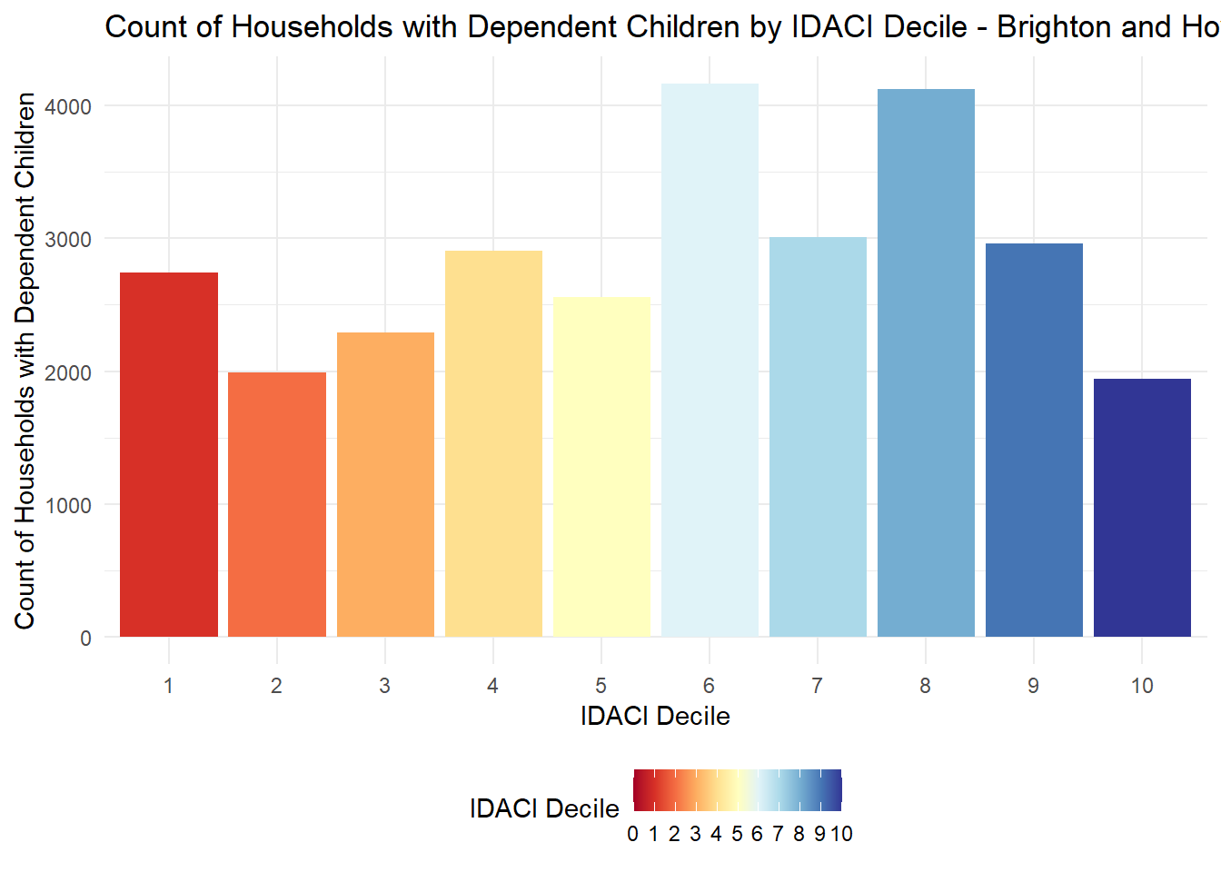
Rayshader Plot

Code
# library(basemaps)
# 
# # Define bounding box for your map area
# # Calculate bounding box explicitly
# bbox <- st_bbox(bn_postcodes_pop1, crs = 4326)
# 
# # set defaults for the basemap
# set_defaults(ext = bbox, map_service = "esri", map_type = "world_light_gray_base")
# 
# # Overlay with your height plot or main plot
# osm_basemap <- ggplot() +
#   basemap_gglayer(ext = bbox) +  # Pass bbox explicitly here
#   scale_fill_identity() +
#   coord_sf()
# 
# 
# osm_basemap
# 
# # Render the rayshader plot with the basemap
# osm_basemap %>%
#   plot_gg(
#     ggobj_height = height_plot,
#     multicore = TRUE,
#     width = 5,
#     height = 5,
#     scale = 50,  # Reduce height scaling
#     windowsize = c(800, 800),
#     shadow_intensity = 0.5  # Optional: adjust shadow for realism
#   )
Code
height_plot <- ggplot(rayshader_data, aes(x = x, y = y, colour = z)) +
  geom_point(size = 0.05) +  # Raster fills for continuous height mapping
  scale_colour_gradientn(
    colors = brewer.pal(9, "YlGnBu"),  # Adjust as needed
    limits = c(min(rayshader_data$z, na.rm = TRUE), max(rayshader_data$z, na.rm = TRUE)),
    name = "Height"
  ) +
  theme_minimal(base_size = 10) +
  labs(
    title = "Households with Dependent Children",
    colour = "IDACI Decile"
  ) +
  theme(
    panel.background = element_rect(fill = "white", color = NA), # White background
    plot.background = element_rect(fill = "white", color = NA),  # White plot background
    legend.background = element_rect(fill = "white", color = NA),
    legend.position = "none"  # Disable all legends# White legend background
  )# Minimal theme for height mapping


#height_plot

main_plot <- ggplot(rayshader_data, aes(x = x, y = y, colour = w)) +
  geom_point(size = 0.05) +
  scale_colour_gradientn(
    colors = brewer.pal(11, "RdYlBu"),
    limits = c(0, 10),
    name = "IDACI Decile"
  ) +
  theme_minimal(base_size = 10) +
  labs(
    title = "IDACI Decile",
    colour = "IDACI Decile"
  ) +
  theme(
    panel.background = element_rect(fill = "white", color = NA), # White background
    plot.background = element_rect(fill = "white", color = NA),  # White plot background
    legend.background = element_rect(fill = "white", color = NA),
    legend.position = "none"  # Disable all legends# White legend background
  )

#main_plot

main_plot %>%
  plot_gg(
    ggobj_height = height_plot,  # Specify height mapping plot
    multicore = TRUE,
    width = 5,
    height = 5,
    scale = 50,  # Adjust scale for height exaggeration
    windowsize = c(1200, 1200), 
    sunangle=225
  )

# Add 3D rendering
render_camera(theta = 10, phi = 30, zoom = 0.4)
rgl::rglwidget()
Code
# 
# bn_bbox = st_bbox(bn_postcodes_pop1)
# 
# bn_roads <- osmdata::opq(bn_bbox) %>% 
#   osmdata::add_osm_feature("highway") %>% 
#   osmdata::osmdata_sf() 
# 
# bn_roads <- bn_roads$osm_lines
# 
# ggplot(bn_roads, aes(color = highway)) + 
#   geom_sf() +
#   theme(legend.position = "none") +
#   labs(title = "Open Street Map `highway` attribute in Brighton")
# 
# rayshader_data_sf <- rayshader_data %>%
#   st_as_sf(coords = c("x", "y"), crs = 4326)
# 
# ggplot(rayshader_data_sf,aes(color=z)) + 
#   geom_sf() +
#   theme(legend.position = "none") 
# 
# map_plot <- ggplot() +
#   geom_sf(data = rayshader_data_sf, aes(color = z)) +
#   geom_sf(data = bn_roads, aes(fill = highway), size = 0.5) +
#   theme_minimal() +
#   theme(
#     panel.background = element_rect(fill = "white", color = NA), # White background
#     plot.background = element_rect(fill = "white", color = NA),  # White plot background
#     legend.background = element_rect(fill = "white", color = NA),
#     legend.position = "none") 
# 
# map_plot %>%
#   plot_gg(
#     ggobj_height = height_plot,  # Specify height mapping plot
#     multicore = TRUE,
#     width = 5,
#     height = 5,
#     scale = 50,  # Adjust scale for height exaggeration
#     windowsize = c(1200, 1200), 
#     sunangle=225
#   )# Disable all legends# White legend
Code
library(sf)
library(dplyr)
library(ggplot2)
library(RColorBrewer)

# Perform spatial join
joined_data_city <- st_join(bn_postcodes_pop1, option0, join = st_within)

# Drop spatial attributes before further operations
joined_data_city <- st_drop_geometry(joined_data_city)

# Aggregate for city-level proportions
city_proportions <- joined_data_city %>%
  group_by(idaci_decile) %>%
  summarise(total_dep_ch = sum(pcd_dep_ch_hh_count_round, na.rm = TRUE)) %>%
  mutate(city_prop = total_dep_ch / sum(total_dep_ch)) %>%
  ungroup()

# Aggregate for catchment-level proportions
catchment_proportions <- joined_data_city %>%
  group_by(catchment, idaci_decile) %>%
  summarise(total_dep_ch = sum(pcd_dep_ch_hh_count_round, na.rm = TRUE)) %>%
  mutate(catchment_prop = total_dep_ch / sum(total_dep_ch)) %>%
  ungroup()
`summarise()` has grouped output by 'catchment'. You can override using the
`.groups` argument.
Code
# Merge city and catchment proportions
# comparison_data <- catchment_proportions %>%
#   left_join(city_proportions %>% select(idaci_decile, city_prop), by = "idaci_decile")

# # Plot proportions comparison
# ggplot(comparison_data, aes(x = factor(idaci_decile))) +
#   geom_bar(aes(y = catchment_prop, fill = "Catchment"), stat = "identity", position = "dodge") +
#   geom_line(aes(y = city_prop, group = 1, color = "City"), size = 1.2) +
#   scale_fill_manual(values = c("Catchment" = "steelblue")) +
#   scale_color_manual(values = c("City" = "darkred")) +
#   labs(
#     title = "Proportions of Households by IDACI Decile",
#     subtitle = "Comparison of Catchment Proportions with City-Level Proportions",
#     x = "IDACI Decile",
#     y = "Proportion of Households",
#     fill = "Legend",
#     color = "Legend"
#   ) +
#   facet_wrap(~ catchment, scales = "free_y") +
#   theme_minimal() +
#   theme(
#     legend.position = "bottom",
#     axis.text.x = element_text(angle = 45, hjust = 1)
#   )
Code
# Initialize an empty data frame to hold the results
comparison_data <- data.frame()

# Get the unique IDACI deciles from city_proportions
unique_deciles <- unique(city_proportions$idaci_decile)

# Loop through each catchment in catchment_proportions
for (catchment in unique(catchment_proportions$catchment)) {
  # Subset data for the current catchment
  catchment_data <- catchment_proportions %>%
    filter(catchment == !!catchment)
  
  # Loop through each IDACI decile
  for (decile in unique_deciles) {
    # Check if the current decile exists in the catchment data
    if (decile %in% catchment_data$idaci_decile) {
      # If it exists, get the proportion for that decile
      catchment_prop <- catchment_data$catchment_prop[catchment_data$idaci_decile == decile]
    } else {
      # If it does not exist, assign a proportion of 0
      catchment_prop <- 0
    }
    
    # Add the current row to the comparison_data
    comparison_data <- rbind(
      comparison_data,
      data.frame(
        catchment = catchment,
        idaci_decile = decile,
        catchment_prop = catchment_prop
      )
    )
  }
}


comparison_data <- comparison_data %>%
  left_join(city_proportions, by = "idaci_decile")

# Add city-level proportions to the data
# comparison_data <- comparison_data %>%
#   left_join(city_proportions %>% select(idaci_decile, city_prop), by = "idaci_decile")

comparison_data <- comparison_data %>%
  mutate(
    diff = catchment_prop - city_prop
  )
Code
ggplot(comparison_data, aes(x = factor(idaci_decile), y = diff, fill = idaci_decile)) +
  geom_bar(stat = "identity") +
  scale_fill_gradientn(
    colors = brewer.pal(11, "RdYlBu"),
    limits = c(0, 10),  # Ensure 0 maps to red and 10 maps to blue
    breaks = 0:10,      # Optional: discrete legend ticks for each decile
    name = "IDACI Decile"
  ) +
  facet_wrap(~ catchment, scales = "fixed") +
  labs(
    title = "Deviation from City Proportion of Deprivation - Current Catchments",
    x = "IDACI Decile",
    y = "Proportion of Households in Catchment"
  ) +
  theme_minimal() +
  theme(legend.position = "bottom") 

 [1] "#808080" "#808080" "#808080" "#808080" "#808080" "#808080" "#808080"
 [8] "#808080" "#808080" "#808080"