Attainment Extras

Executive Summary

• Following on analysis from my last piece on the importance of absence, this work verifies that posted by Ben Harper on Facebook and shows that for schools in the range of levels of disadvantage that Brighton and Hove experiences, there is NO RELATIONSHIP between attainment, progress and school-level disadvantage concentrations. NO RELATIONSHIP.

• Even if there was no negative collateral damage caused by forcing thousands of children to attend schools outside of their catchment area to affect changes in the proportions of disadvantage in different schools in the city (and there will be lots of negative collateral damage), the evidence from this analysis is there will be NO BENEFIT to disadvantaged attainment of changes to school-level disadvantage concentrations. None.

• Having examined the original Stephen Gorard paper where the idea for increased social mixing having a positive effect on attainment first emerged, the authors themselves only cite a weak effect from social mixing on attainment. But having identified clear non-linearities in the relationship between attainment and disadvantage at the national school level in the DfE 2022-23 data (see all of the plots below), without verifiable data plots and other indicative regression diagnostics in the Gorard paper, it is possible that the weak linear relationship reported at the national level is not reliable - there is a good chance that it is violating standard linear regression assumptions.

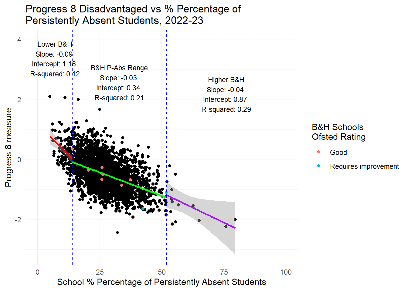
• While there is no relationship between concentrations of disadvantage and levels of disadvantaged attainment in the Brighton and Hove range, the evidence below suggests strongly that if persistent absence were reduced - even just for schools in the range of persistent absence that Brighton and Hove experiences - noticeable improvements in disadvantaged attainment could be achieved.

• In the face of this evidence against any effects at all, can the council continue to justify a policy - specifically the 20% open allocation policy which would lead to 20% of the places in a catchment being allocated to out of catchment children, resulting in the displacement of 10% of students in the city outside of their catchment - on the grounds of trying to improve attainment through mixing?

• In the face of this evidence, can the council explain why it has not switched its focus to tackling persistent absence in the city and why it has not announced that it will not be pursuing the 20% open ballot policy given the overwhelming likelihood of no positive effects on disadvantaged attainment and significant and numerous negative effects?

Overview

Science and Policy

All good science proceeds incrementally and builds on the excellent work of others through reproducibility coupled with new perspectives and ideas often brought from other disciplines, societies and cultures. Science is not perfect, but for all of its faults its the best system humans have developed for advancing humanity’s understanding of the world. And to be fair, it has achieved a fair amount in a pretty short space of time.

All good policy is evidence-based policy - and to borrow the wikipedia definition (for it is both accessible and good):

An individual or organisation is justified in claiming that a specific policy is evidence-based if, and only if, three conditions are met:

1. the individual or organisation possesses comparative evidence about the effects of the specific policy in comparison to the effects of at least one alternative policy

2. the specific policy is supported by this evidence according to at least one of the individual’s or organisation’s preferences in the given policy area

3. the individual or organisation can provide a sound account for this support by explaining the evidence and preferences that lay the foundation for the claim

The darker, always less successful opposite to evidence-based policy is policy-based evidence making. We can probably all think of examples, but this is where someone might observe something, decide on what they think the best course of action is, formulate a policy to make that thing happen, and then search around to find some evidence to post-hoc justify that policy to people they might have to justify it too.

Right back at the beginning of the engagement exercise last year, the council stated that its ambitions for the re-organisation of the school admissions system were ‘evidence based’. Since then, much more evidence has arrived that call that into question. Here is some more.

Science and Reproducibility

Returning to science - in the same way that I apparently inspired some work that Ben Harper posted on Facebook here. I have been inspired to verify and build on this work.

That first post was then also followed with another post here where the the relative weakness of the Gorardian association between social mixing and attainment first cited in this paper was highlighted. A factor at the national level - albeit a weak one even acknowledged by the authors.

Harper’s crucial insight after seeing the non-linear relationship in my work was that Gorard’s weak negative relationship between attainment and disadvantage (leaving aside the chance that the relationship might be in violation of the assumptions of linearity that underpin their validity) might be even weaker if we restrict our analysis to the reality of Brighton and Hove.

This is really important. Brighton is a medium sized city and like every other town and city of a reasonable size in the country, has pockets of wealth and affluence. As such, it will never attain the kind of low-levels of disadvantage you might find, say, in a leafy commuter town in Surrey. And because the town does already have relatively well mixed schools in the state sector, it will never have schools with levels of disadvantage lower than the lowest level experienced at the moment while the city-wide levels of disadvantage are projected to increase in the future. If city-wide levels come down, then some schools may also reduce.

These insights from Harper are crucial important as they provide strong evidence that for disadvantaged students (those who BHCC have identified as wanting to improve attainment for), no amount of increased or decreased social mixing in schools will make a difference to their progress or attainment at the end of KS4.

In the spirit of reproducibility, I have had a go at reproducing Harper’s plots and have extended them a little and looked also at persistent absence as a contract. To be clear: Using data from 2022-23 for all state secondary schools in England, for the range of disadvantage experienced in Brighton and Hove Schools (and we know that levels of disadvantage in the city are likely to increase overall from the Council’s own projections), I agree with Harper that there is NO RELATIONSHIP between the increase or decrease in the total proportion of disadvantaged pupils in those schools and the increase or decrease or both Progress 8 and Attainment 8 scores. NO RELATIONSHIP.

There is a weak negative relationship for non-disadvantaged students. This means that through a policy of increased social mixing - even before we try to account for the negative impacts of increased travel which will be used to facilitate the mixing - we can predict that the council might well be successful in reducing the attainment gap in the city, but only through reducing, slightly, the attainment of non-disadvantaged students in those schools where disadvantaged proportions increase. The gap won’t be closed through increasing the attainment of disadvantaged students - this is likely to remain static.

HOWEVER, it is a different story altogether when we look at persistent absence. If you had read my last piece here you might already be guessing where this is going. Yes, there is a STONG RELATIONSHIP between persistent absence and attainment in the range Brighton and Hove experiences. It is closer to a linear relationship for Progress 8 anyway, but also holds for Attainment 8 which is not a linear relationship, but pretty linear for the Brighton and Hove range.

What is interesting is that the plots below actually corroborate the weak negative associations (and at about the same level - although in Gorard’s paper they use standardised coefficients and don’t provide the raw outputs so we can’t match directly coefficient values) between attainment and disadvantage if we assume a linear relationship. But as the plots show clearly and as Ben Harper pointed out before, this is NOT a linear relationship - and as anyone with undergraduate level training in statistics will tell you, for the coefficients in a linear relationship to be valid and reliable, the variables must have a linear association. So there is strong evidence here - and Gorard’s paper doesn’t provide the kind of visual outputs or regression diagnostics we need to check this for sure - that the big association trumpeted by the council between attainment and concentrations of disadvantage - is neither big nor relevant for schools exhibiting the levels of disadvantage we do in Brighton.

I will therefore repeat what I said before: If Brighton and Hove Council are serious about wanting to improve the attainment of disadvantaged students in the city, they will not achieve this through changing the concentrations of disadvantage in the schools in the city. Even if all schools had the ‘city average’ for FSM concentrations, the evidence looking at all schools in England is there would be no benefit for the attainment disadvantaged pupils. However, if the council focused on reducing levels of persistent absence, there would be a strong likelihood that the attainment of those pupils would improve - disadvantaged or non-disadvantaged alike.

Explore the plots below if you would like to see this for yourself.

What does this mean for evidence-based policy?

1. the individual or organisation possesses comparative evidence about the effects of the specific policy in comparison to the effects of at least one alternative policy

The plots below compare the effects of adjusting levels of disadvantage in schools with adjusting levels of persistent absence in schools on their levels of attainment and progress. This is comparative evidence.

Adjusting levels of disadvantage in the range that Brighton and Hove experiences has NO EFFECT on attainment.

Adjusting levels of persistent absence has quite a large effect on attainment.

Which might be the more sensible policy target to pursue? Levels of disadvantage or levels of persistent absence?

2. the specific policy is supported by this evidence according to at least one of the individual’s or organisation’s preferences in the given policy area

BHCC clearly has a preference to try and affect change in attainment for disadvantaged pupils through adjusting levels of disadvantage in schools. This work has shown that the evidence this preference is built upon is likely to be flawed (a linear coefficient cited for a non-linear relationship at the national level). Restricting the analysis to the reality of disadvantage in Brighton, it has also shown that for Brighton the any relationship between school-level disadvantage and school-level attainment for disadvantaged pupils, disappears.

3. the individual or organisation can provide a sound account for this support by explaining the evidence and preferences that lay the foundation for the claim

Given the evidence below and in my last piece, can BHCC provide a sound account for supporting a policy to try and improve disadvantaged attainment based on socially engineering new concentrations of disadvantage in schools - even leaving aside the huge negative impacts such a policy might entail - when it is clear the evidence for an effect is non-existent?

Can they justify why a new policy based on reducing the levels of persistent absence in the city is not being disucssed or promoted to the community?

library(tidyverse)
library(here)
library(janitor)
library(sf)

##Absence 2022-23 regression analysis

##All Data downloaded from here
##https://www.compare-school-performance.service.gov.uk/

#read in data for every school in the country

england_abs <- read_csv(here("data", "Performancetables_Eng_2022_23", "2022-2023", "england_abs.csv"), na = c("", "NA", "SUPP", "NP", "NE"))
england_census <- read_csv(here("data", "Performancetables_Eng_2022_23", "2022-2023", "england_census.csv"), na = c("", "NA", "SUPP", "NP", "NE"))
england_ks4final <- read_csv(here("data", "Performancetables_Eng_2022_23", "2022-2023", "england_ks4final.csv"), na = c("", "NA", "SUPP", "NP", "NE"))
england_school_information <- read_csv(here("data", "Performancetables_Eng_2022_23", "2022-2023", "england_school_information.csv"), na = c("", "NA", "SUPP", "NP", "NE"))

england_ks4final <- england_ks4final %>%
  mutate(URN = as.character(URN)) %>%
  mutate(across(TOTPUPS:PTOTENT_E_COVID_IMPACTED_PTQ_EE, ~ parse_number(as.character(.))))

england_ks4final <- england_ks4final %>%
  filter(!is.na(URN))

england_abs <- england_abs %>%
  mutate(URN = as.character(URN))

england_census <- england_census %>%
  mutate(URN = as.character(URN))

england_school_information <- england_school_information %>%
  mutate(URN = as.character(URN))

# Left join england_ks4final with england_abs
england_school_2022_23 <- england_ks4final %>%
  left_join(england_abs, by = "URN") %>%
  left_join(england_census, by = "URN") %>%
  left_join(england_school_information, by = "URN")

data_types <- sapply(england_school_2022_23, class)
england_school_2022_23_meta <- data.frame(Field = names(data_types), DataType = data_types)

Disadvantage

Attainment 8

Attainment Non-Disadvantaged All

# Calculate the min and max values for the subset range
min_value <- min(btn_sub$PTFSM6CLA1A, na.rm = TRUE)
max_value <- max(btn_sub$PTFSM6CLA1A, na.rm = TRUE)

# Fit the linear model for the entire data
lm_model <- lm(ATT8SCR_NFSM6CLA1A ~ PTFSM6CLA1A, data = england_school_2022_23_not_special)
lm_summary <- summary(lm_model)
slope <- lm_summary$coefficients[2, 1]
intercept <- lm_summary$coefficients[1, 1]
r_squared <- lm_summary$r.squared

# Annotation text
annotation_text <- paste("Slope:", round(slope, 2), "\nIntercept:", round(intercept, 2), "\nR-squared:", round(r_squared, 2))

# Plot the data with a linear regression line and annotation
ggplot(england_school_2022_23_not_special, aes(y = ATT8SCR_NFSM6CLA1A, x = PTFSM6CLA1A)) +
  geom_point() +
  geom_point(data = btn_sub, aes(y = ATT8SCR_NFSM6CLA1A, x = PTFSM6CLA1A, colour = OFSTEDRATING)) +
  geom_vline(xintercept = min_value, linetype = "dashed", color = "blue") +
  geom_vline(xintercept = max_value, linetype = "dashed", color = "blue") +
  geom_smooth(method = "lm", se = TRUE, color = "red") +
  labs(title = "Attainment 8 Non-Disadvantaged vs % School Percentage of \nDisadvantaged Students, 2022-23",
       x = "% Percentage of Disadvantaged Students",
       y = "Attainment 8 measure",
       color = "B&H Schools \nOfsted Rating") +
  theme_minimal() +
  xlim(0, 100) +
  annotate("text", x = 80, y = min(england_school_2022_23_not_special$ATT8SCR_NFSM6CLA1A, na.rm = TRUE), 
           label = annotation_text, hjust = 1, vjust = 0, size = 3)

Attainment Non-Disadvantaged B&H Range

# Calculate the min and max values for the subset range
min_value <- min(btn_sub$PTFSM6CLA1A, na.rm = TRUE)
max_value <- max(btn_sub$PTFSM6CLA1A, na.rm = TRUE)

# Create the subset
subset_data <- england_school_2022_23_not_special %>%
  filter(PTFSM6CLA1A >= min_value & PTFSM6CLA1A <= max_value)

# Fit the linear model
lm_model <- lm(ATT8SCR_NFSM6CLA1A ~ PTFSM6CLA1A, data = subset_data)
lm_summary <- summary(lm_model)
slope <- lm_summary$coefficients[2, 1]
intercept <- lm_summary$coefficients[1, 1]
r_squared <- lm_summary$r.squared

# Annotation text
annotation_text <- paste("Slope:", round(slope, 2), "\nIntercept:", round(intercept, 2), "\nR-squared:", round(r_squared, 2))

# Plot the data with a linear regression line and annotation
ggplot(subset_data, aes(y = ATT8SCR_NFSM6CLA1A, x = PTFSM6CLA1A)) +
  geom_point() +
  geom_point(data = btn_sub, aes(y = ATT8SCR_NFSM6CLA1A, x = PTFSM6CLA1A, colour = OFSTEDRATING)) +
  geom_vline(xintercept = min_value, linetype = "dashed", color = "blue") +
  geom_vline(xintercept = max_value, linetype = "dashed", color = "blue") +
  geom_smooth(method = "lm", se = TRUE, color = "red") +
  labs(title = "Attainment Non-Disadvantaged 8 vs % Percentage of \nDisadvantaged Students, 2022-23",
       x = "% Percentage of Disadvantaged Students",
       y = "Attainment 8 measure",
       color = "B&H Schools \nOfsted Rating") +
  theme_minimal() +
  xlim(0, 100) +
  annotate("text", x = 80, y = min(subset_data$ATT8SCR_NFSM6CLA1A, na.rm = TRUE), 
           label = annotation_text, hjust = 1, vjust = 0, size = 3)

Attainment Non-Disadvantaged Mixed Ranges

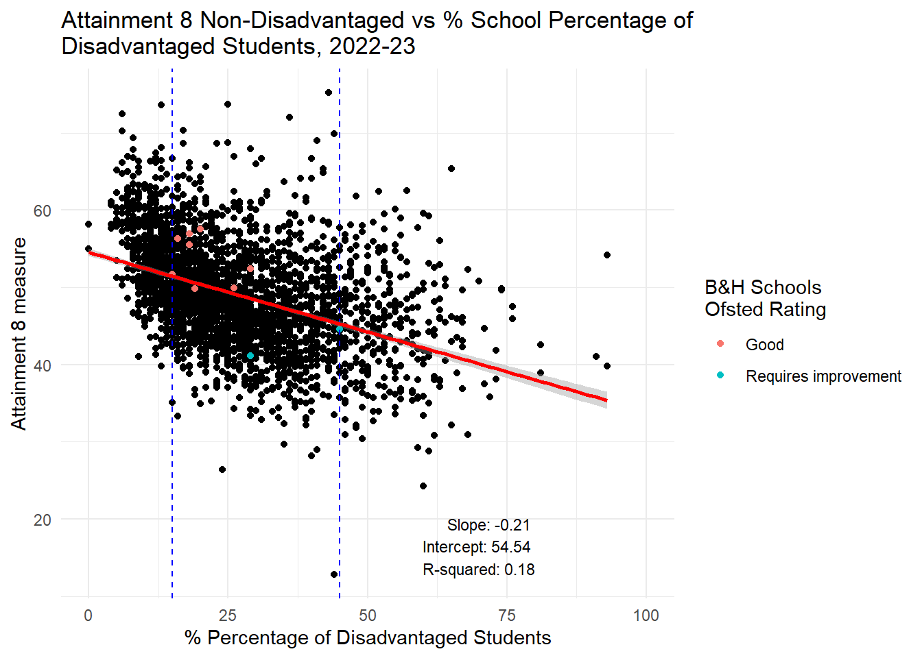
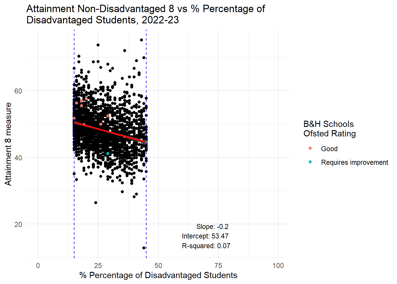
# Calculate the min and max values for the subset range
min_value <- min(btn_sub$PTFSM6CLA1A, na.rm = TRUE)
max_value <- max(btn_sub$PTFSM6CLA1A, na.rm = TRUE)

# Create subsets
subset_before <- england_school_2022_23_not_special %>%
  filter(PTFSM6CLA1A < min_value)

subset_after <- england_school_2022_23_not_special %>%
  filter(PTFSM6CLA1A > max_value)

subset_within <- england_school_2022_23_not_special %>%
  filter(PTFSM6CLA1A >= min_value & PTFSM6CLA1A <= max_value)

# Fit linear models
lm_before <- lm(ATT8SCR_NFSM6CLA1A ~ PTFSM6CLA1A, data = subset_before)
lm_within <- lm(ATT8SCR_NFSM6CLA1A ~ PTFSM6CLA1A, data = subset_within)
lm_after <- lm(ATT8SCR_NFSM6CLA1A ~ PTFSM6CLA1A, data = subset_after)

# Calculate middle x positions for annotations
middle_before <- mean(c(0, min_value))
middle_within <- mean(c(min_value, max_value))
middle_after <- mean(c(max_value, 100))

# Plot the data with annotations
ggplot(england_school_2022_23_not_special, aes(y = ATT8SCR_NFSM6CLA1A, x = PTFSM6CLA1A)) +
  geom_point() +
  geom_point(data = btn_sub, aes(y = ATT8SCR_NFSM6CLA1A, x = PTFSM6CLA1A, colour = OFSTEDRATING)) +
  geom_vline(xintercept = min_value, linetype = "dashed", color = "blue") +
  geom_vline(xintercept = max_value, linetype = "dashed", color = "blue") +
  geom_smooth(data = subset_before, method = "lm", se = TRUE, color = "red", linetype = "solid", aes(group = 1)) +
  geom_smooth(data = subset_within, method = "lm", se = TRUE, color = "green", linetype = "solid", aes(group = 1)) +
  geom_smooth(data = subset_after, method = "lm", se = TRUE, color = "purple", linetype = "solid", aes(group = 1)) +
  labs(title = "Attainment 8 Non-Disadvantaged vs % Percentage of \nDisadvantaged Students, 2022-23",
       x = "School % Percentage of Disadvantaged Students",
       y = "Attainment 8 measure",
       color = "B&H Schools \nOfsted Rating") +
  theme_minimal() +
  xlim(0, 100) +
  annotate("text", x = middle_before, y = min(subset_before$ATT8SCR_NFSM6CLA1A, na.rm = TRUE) + 5, 
           label = paste("Lower B&H\nSlope:", round(coef(lm_before)[2], 2),
                         "\nIntercept:", round(coef(lm_before)[1], 2),
                         "\nR-squared:", round(summary(lm_before)$r.squared, 2)), 
           hjust = 0.5, vjust = 0, size = 3) +
  annotate("text", x = middle_within, y = min(subset_within$ATT8SCR_NFSM6CLA1A, na.rm = TRUE) + 5, 
           label = paste("B&H FSM Range\nSlope:", round(coef(lm_within)[2], 2),
                         "\nIntercept:", round(coef(lm_within)[1], 2),
                         "\nR-squared:", round(summary(lm_within)$r.squared, 2)), 
           hjust = 0.5, vjust = 1, size = 3) +
  annotate("text", x = middle_after, y = min(subset_after$ATT8SCR_NFSM6CLA1A, na.rm = TRUE) + 5, 
           label = paste("Higher B&H\nSlope:", round(coef(lm_after)[2], 2),
                         "\nIntercept:", round(coef(lm_after)[1], 2),
                         "\nR-squared:", round(summary(lm_after)$r.squared, 2)), 
           hjust = 0.5, vjust = 1, size = 3)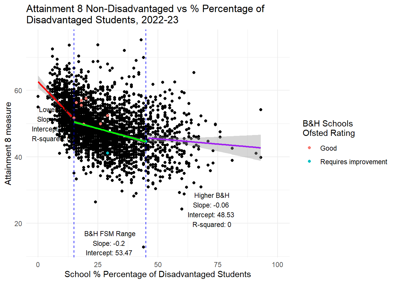

Attainment Disadvantaged All

# Calculate the min and max values for the subset range
min_value <- min(btn_sub$PTFSM6CLA1A, na.rm = TRUE)
max_value <- max(btn_sub$PTFSM6CLA1A, na.rm = TRUE)

# Fit the linear model for the entire data
lm_model <- lm(ATT8SCR_FSM6CLA1A ~ PTFSM6CLA1A, data = england_school_2022_23_not_special)
lm_summary <- summary(lm_model)
slope <- lm_summary$coefficients[2, 1]
intercept <- lm_summary$coefficients[1, 1]
r_squared <- lm_summary$r.squared

# Annotation text
annotation_text <- paste("Slope:", round(slope, 2), "\nIntercept:", round(intercept, 2), "\nR-squared:", round(r_squared, 2))

# Plot the data with a linear regression line and annotation
ggplot(england_school_2022_23_not_special, aes(y = ATT8SCR_FSM6CLA1A, x = PTFSM6CLA1A)) +
  geom_point() +
  geom_point(data = btn_sub, aes(y = ATT8SCR_FSM6CLA1A, x = PTFSM6CLA1A, colour = OFSTEDRATING)) +
  geom_vline(xintercept = min_value, linetype = "dashed", color = "blue") +
  geom_vline(xintercept = max_value, linetype = "dashed", color = "blue") +
  geom_smooth(method = "lm", se = TRUE, color = "red") +
  labs(title = "Attainment 8 Disadvantaged vs % School Percentage of \nDisadvantaged Students, 2022-23",
       x = "% Percentage of Disadvantaged Students",
       y = "Attainment 8 measure",
       color = "B&H Schools \nOfsted Rating") +
  theme_minimal() +
  xlim(0, 100) +
  annotate("text", x = 80, y = min(england_school_2022_23_not_special$ATT8SCR_FSM6CLA1A, na.rm = TRUE), 
           label = annotation_text, hjust = 1, vjust = 0, size = 3)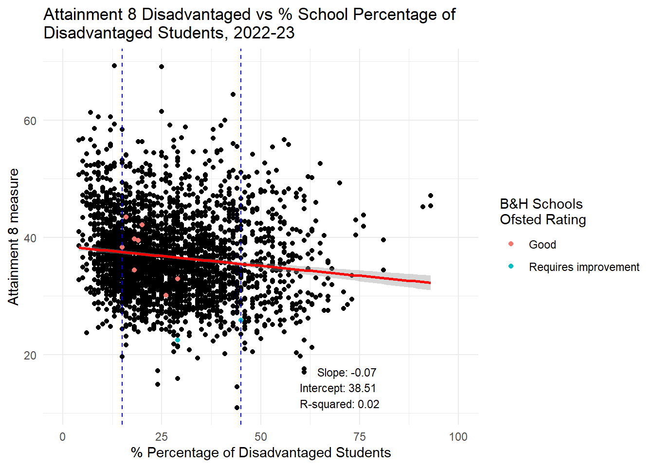

Attainment Disadvantaged B&H Range

# Calculate the min and max values for the subset range
min_value <- min(btn_sub$PTFSM6CLA1A, na.rm = TRUE)
max_value <- max(btn_sub$PTFSM6CLA1A, na.rm = TRUE)

# Create the subset
subset_data <- england_school_2022_23_not_special %>%
  filter(PTFSM6CLA1A >= min_value & PTFSM6CLA1A <= max_value)

# Fit the linear model
lm_model <- lm(ATT8SCR_FSM6CLA1A ~ PTFSM6CLA1A, data = subset_data)
lm_summary <- summary(lm_model)
slope <- lm_summary$coefficients[2, 1]
intercept <- lm_summary$coefficients[1, 1]
r_squared <- lm_summary$r.squared

# Annotation text
annotation_text <- paste("Slope:", round(slope, 2), "\nIntercept:", round(intercept, 2), "\nR-squared:", round(r_squared, 2))

# Plot the data with a linear regression line and annotation
ggplot(subset_data, aes(y = ATT8SCR_FSM6CLA1A, x = PTFSM6CLA1A)) +
  geom_point() +
  geom_point(data = btn_sub, aes(y = ATT8SCR_FSM6CLA1A, x = PTFSM6CLA1A, colour = OFSTEDRATING)) +
  geom_vline(xintercept = min_value, linetype = "dashed", color = "blue") +
  geom_vline(xintercept = max_value, linetype = "dashed", color = "blue") +
  geom_smooth(method = "lm", se = TRUE, color = "red") +
  labs(title = "Attainment Disadvantaged 8 vs % Percentage of \nDisadvantaged Students, 2022-23",
       x = "% Percentage of Disadvantaged Students",
       y = "Attainment 8 measure",
       color = "B&H Schools \nOfsted Rating") +
  theme_minimal() +
  xlim(0, 100) +
  annotate("text", x = 80, y = min(subset_data$ATT8SCR_FSM6CLA1A, na.rm = TRUE), 
           label = annotation_text, hjust = 1, vjust = 0, size = 3)

Attainment Disadvantaged Mixed Ranges

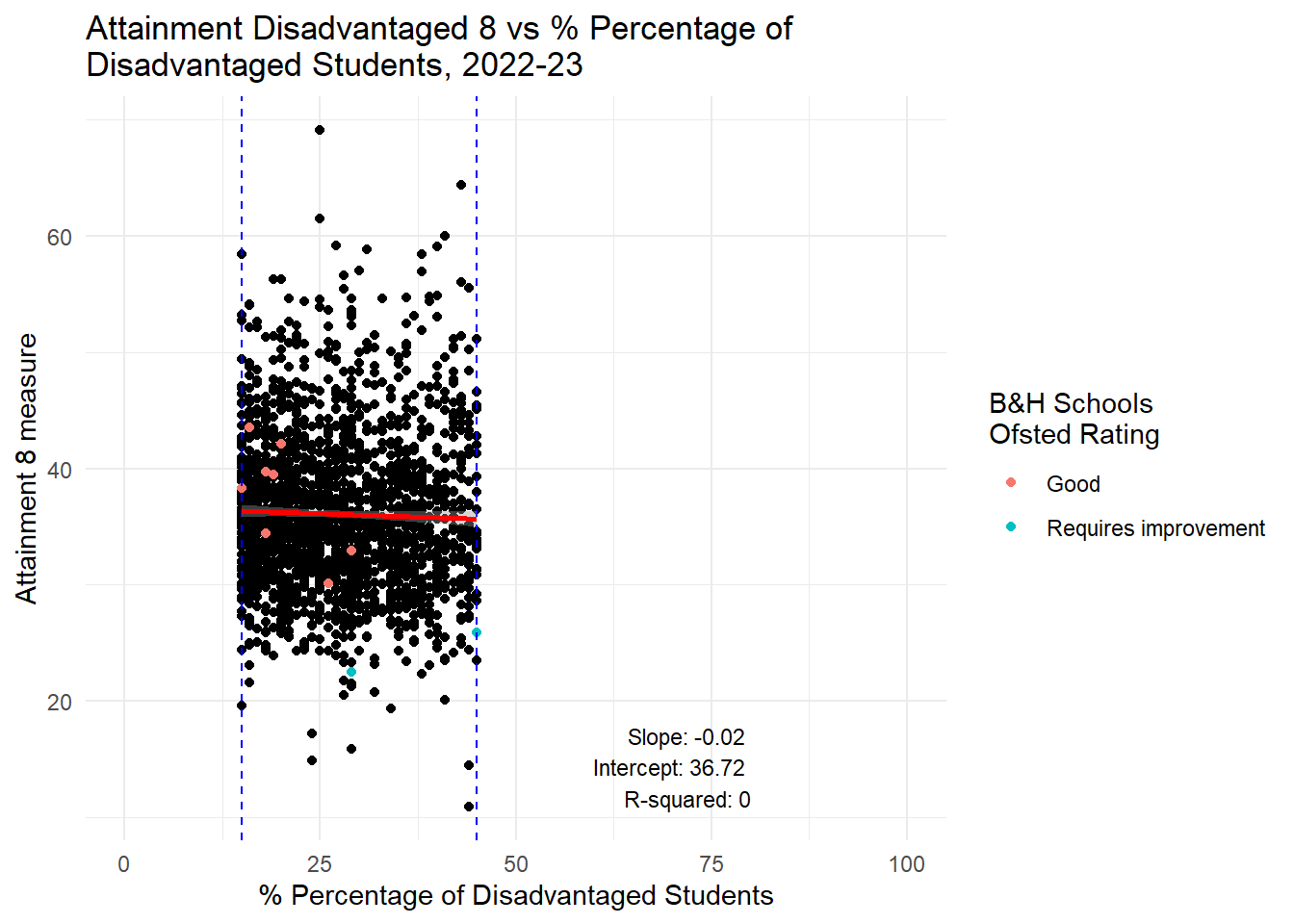
# Calculate the min and max values for the subset range
min_value <- min(btn_sub$PTFSM6CLA1A, na.rm = TRUE)
max_value <- max(btn_sub$PTFSM6CLA1A, na.rm = TRUE)

# Create subsets
subset_before <- england_school_2022_23_not_special %>%
  filter(PTFSM6CLA1A < min_value)

subset_after <- england_school_2022_23_not_special %>%
  filter(PTFSM6CLA1A > max_value)

subset_within <- england_school_2022_23_not_special %>%
  filter(PTFSM6CLA1A >= min_value & PTFSM6CLA1A <= max_value)

# Fit linear models
lm_before <- lm(ATT8SCR_FSM6CLA1A ~ PTFSM6CLA1A, data = subset_before)
lm_within <- lm(ATT8SCR_FSM6CLA1A ~ PTFSM6CLA1A, data = subset_within)
lm_after <- lm(ATT8SCR_FSM6CLA1A ~ PTFSM6CLA1A, data = subset_after)

# Calculate middle x positions for annotations
middle_before <- mean(c(0, min_value))
middle_within <- mean(c(min_value, max_value))
middle_after <- mean(c(max_value, 100))

# Plot the data with annotations
ggplot(england_school_2022_23_not_special, aes(y = ATT8SCR_FSM6CLA1A, x = PTFSM6CLA1A)) +
  geom_point() +
  geom_point(data = btn_sub, aes(y = ATT8SCR_FSM6CLA1A, x = PTFSM6CLA1A, colour = OFSTEDRATING)) +
  geom_vline(xintercept = min_value, linetype = "dashed", color = "blue") +
  geom_vline(xintercept = max_value, linetype = "dashed", color = "blue") +
  geom_smooth(data = subset_before, method = "lm", se = TRUE, color = "red", linetype = "solid", aes(group = 1)) +
  geom_smooth(data = subset_within, method = "lm", se = TRUE, color = "green", linetype = "solid", aes(group = 1)) +
  geom_smooth(data = subset_after, method = "lm", se = TRUE, color = "purple", linetype = "solid", aes(group = 1)) +
  labs(title = "Attainment 8 Disadvantaged vs % Percentage of \nDisadvantaged Students, 2022-23",
       x = "School % Percentage of Disadvantaged Students",
       y = "Attainment 8 measure",
       color = "B&H Schools \nOfsted Rating") +
  theme_minimal() +
  xlim(0, 100) +
  annotate("text", x = middle_before, y = min(subset_before$ATT8SCR_FSM6CLA1A, na.rm = TRUE) + 5, 
           label = paste("Lower B&H\nSlope:", round(coef(lm_before)[2], 2),
                         "\nIntercept:", round(coef(lm_before)[1], 2),
                         "\nR-squared:", round(summary(lm_before)$r.squared, 2)), 
           hjust = 0.5, vjust = 1.5, size = 3) +
  annotate("text", x = middle_within, y = min(subset_within$ATT8SCR_FSM6CLA1A, na.rm = TRUE) + 5, 
           label = paste("B&H FSM Range\nSlope:", round(coef(lm_within)[2], 2),
                         "\nIntercept:", round(coef(lm_within)[1], 2),
                         "\nR-squared:", round(summary(lm_within)$r.squared, 2)), 
           hjust = 0.75, vjust = -4, size = 3) +
  annotate("text", x = middle_after, y = min(subset_after$ATT8SCR_FSM6CLA1A, na.rm = TRUE) + 5, 
           label = paste("Higher B&H\nSlope:", round(coef(lm_after)[2], 2),
                         "\nIntercept:", round(coef(lm_after)[1], 2),
                         "\nR-squared:", round(summary(lm_after)$r.squared, 2)), 
           hjust = 0.5, vjust = -2.5, size = 3)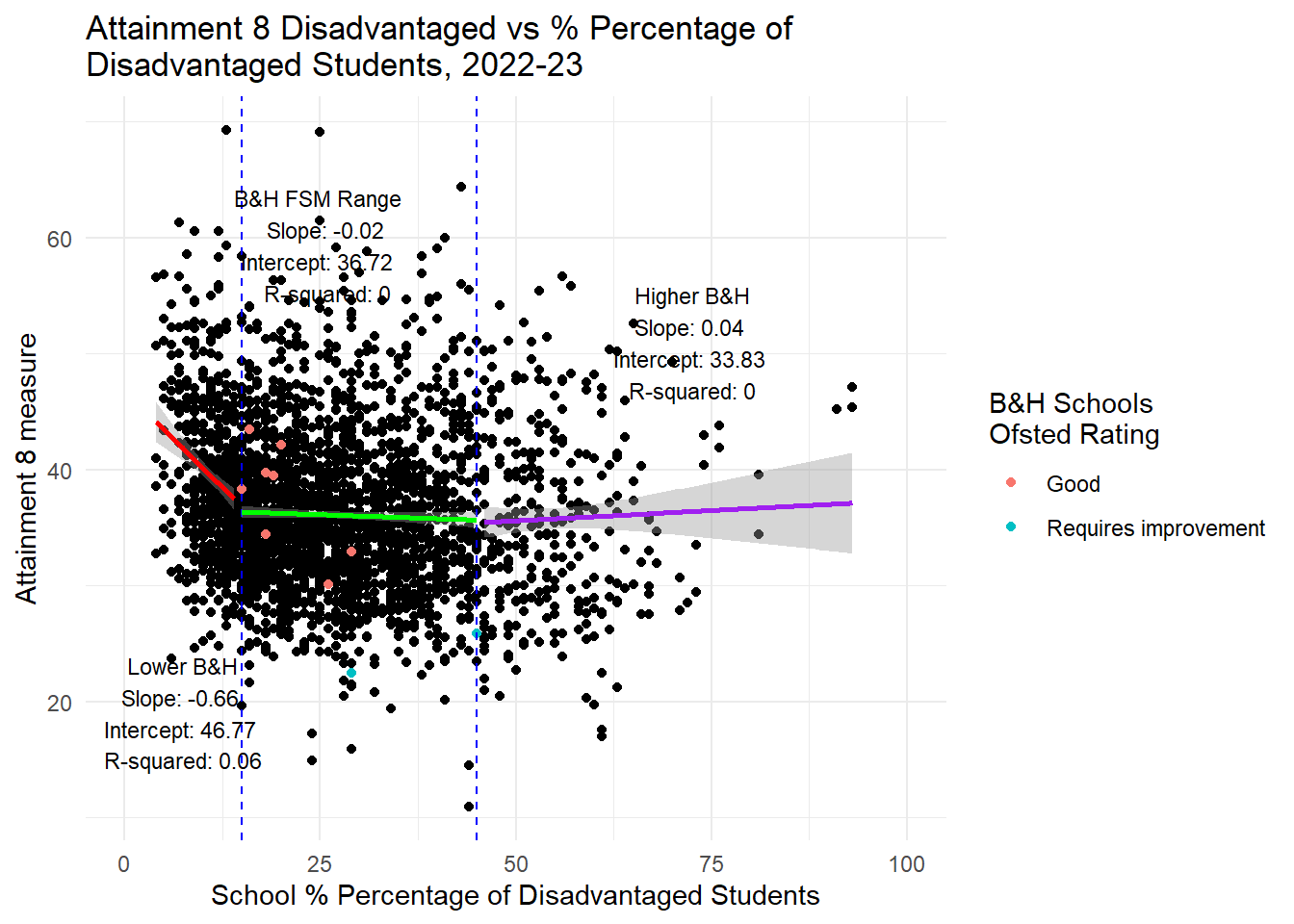

#ggsave(here("images", "Attainment8_disadvantage.png"))

Progress 8

Progress Non-Disadvantaged All

# Calculate the min and max values for the subset range
min_value <- min(btn_sub$PTFSM6CLA1A, na.rm = TRUE)
max_value <- max(btn_sub$PTFSM6CLA1A, na.rm = TRUE)

# Fit the linear model for the entire data
lm_model <- lm(P8MEA_NFSM6CLA1A ~ PTFSM6CLA1A, data = england_school_2022_23_not_special)
lm_summary <- summary(lm_model)
slope <- lm_summary$coefficients[2, 1]
intercept <- lm_summary$coefficients[1, 1]
r_squared <- lm_summary$r.squared

# Annotation text
annotation_text <- paste("Slope:", round(slope, 2), "\nIntercept:", round(intercept, 2), "\nR-squared:", round(r_squared, 2))

# Plot the data with a linear regression line and annotation
ggplot(england_school_2022_23_not_special, aes(y = P8MEA_NFSM6CLA1A, x = PTFSM6CLA1A)) +
  geom_point() +
  geom_point(data = btn_sub, aes(y = P8MEA_NFSM6CLA1A, x = PTFSM6CLA1A, colour = OFSTEDRATING)) +
  geom_vline(xintercept = min_value, linetype = "dashed", color = "blue") +
  geom_vline(xintercept = max_value, linetype = "dashed", color = "blue") +
  geom_smooth(method = "lm", se = TRUE, color = "red") +
  labs(title = "Progress 8 Non-Disadvantaged vs % School Percentage of \nDisadvantaged Students, 2022-23",
       x = "% Percentage of Disadvantaged Students",
       y = "Progress 8 measure",
       color = "B&H Schools \nOfsted Rating") +
  theme_minimal() +
  xlim(0, 100) +
  annotate("text", x = 80, y = min(england_school_2022_23_not_special$P8MEA_NFSM6CLA1A, na.rm = TRUE), 
           label = annotation_text, hjust = 1, vjust = 0, size = 3)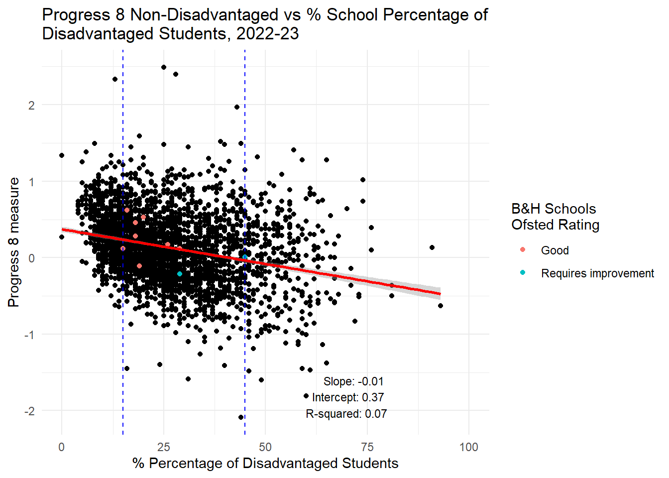

Progress Non-Disadvantaged B&H Range

# Calculate the min and max values for the subset range
min_value <- min(btn_sub$PTFSM6CLA1A, na.rm = TRUE)
max_value <- max(btn_sub$PTFSM6CLA1A, na.rm = TRUE)

# Create the subset
subset_data <- england_school_2022_23_not_special %>%
  filter(PTFSM6CLA1A >= min_value & PTFSM6CLA1A <= max_value)

# Fit the linear model
lm_model <- lm(P8MEA_NFSM6CLA1A ~ PTFSM6CLA1A, data = subset_data)
lm_summary <- summary(lm_model)
slope <- lm_summary$coefficients[2, 1]
intercept <- lm_summary$coefficients[1, 1]
r_squared <- lm_summary$r.squared

# Annotation text
annotation_text <- paste("Slope:", round(slope, 2), "\nIntercept:", round(intercept, 2), "\nR-squared:", round(r_squared, 2))

# Plot the data with a linear regression line and annotation
ggplot(subset_data, aes(y = P8MEA_NFSM6CLA1A, x = PTFSM6CLA1A)) +
  geom_point() +
  geom_point(data = btn_sub, aes(y = P8MEA_NFSM6CLA1A, x = PTFSM6CLA1A, colour = OFSTEDRATING)) +
  geom_vline(xintercept = min_value, linetype = "dashed", color = "blue") +
  geom_vline(xintercept = max_value, linetype = "dashed", color = "blue") +
  geom_smooth(method = "lm", se = TRUE, color = "red") +
  labs(title = "Progress 8 Non-Disadvantaged vs % Percentage of \nDisadvantaged Students, 2022-23",
       x = "% Percentage of Disadvantaged Students",
       y = "Progress 8 measure",
       color = "B&H Schools \nOfsted Rating") +
  theme_minimal() +
  xlim(0, 100) +
  annotate("text", x = 80, y = min(subset_data$P8MEA_NFSM6CLA1A, na.rm = TRUE), 
           label = annotation_text, hjust = 1, vjust = 0, size = 3)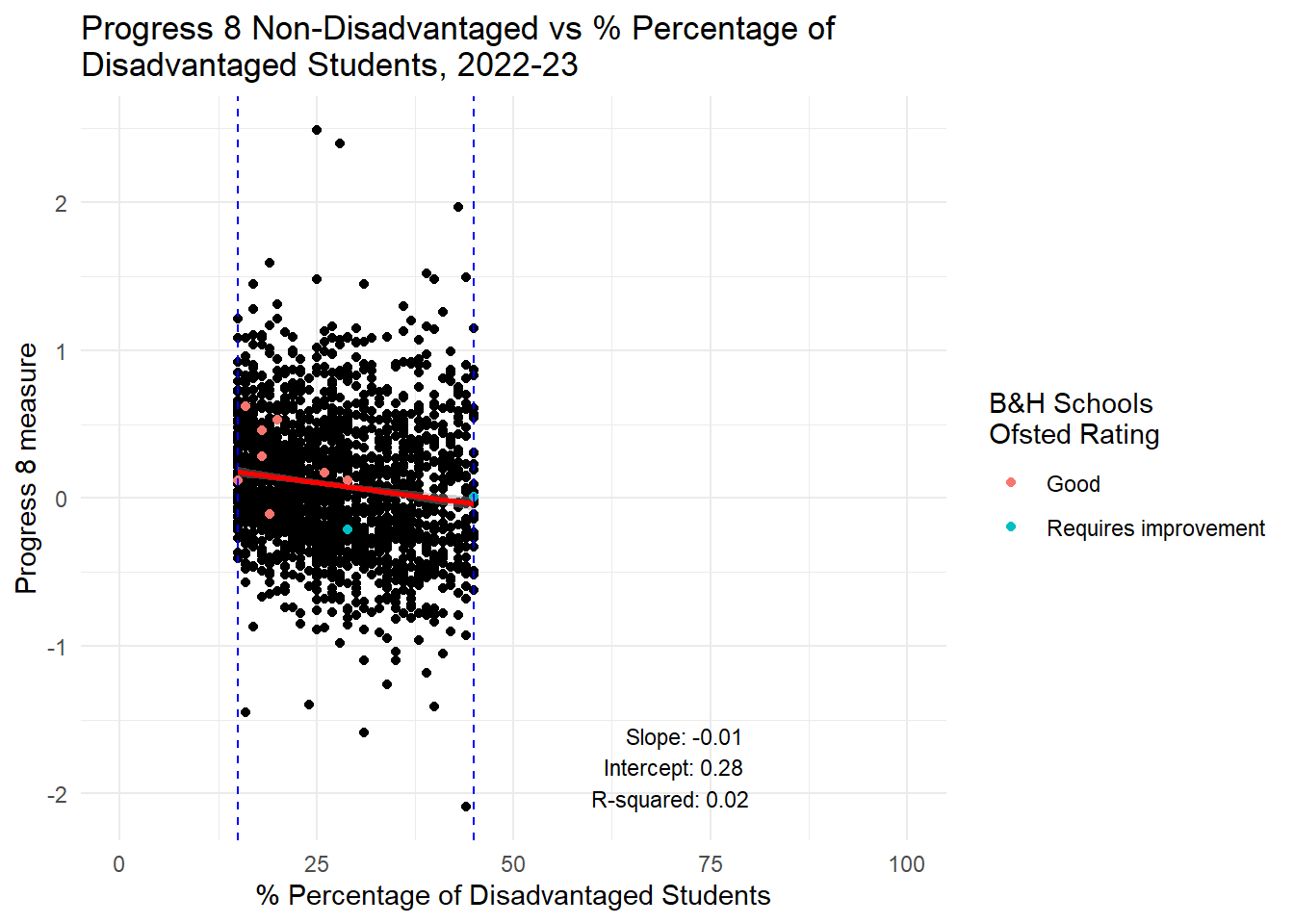

Progress Non-Disadvantaged Mixed Ranges

# Calculate the min and max values for the subset range
min_value <- min(btn_sub$PTFSM6CLA1A, na.rm = TRUE)
max_value <- max(btn_sub$PTFSM6CLA1A, na.rm = TRUE)

# Create subsets
subset_before <- england_school_2022_23_not_special %>%
  filter(PTFSM6CLA1A < min_value)

subset_after <- england_school_2022_23_not_special %>%
  filter(PTFSM6CLA1A > max_value)

subset_within <- england_school_2022_23_not_special %>%
  filter(PTFSM6CLA1A >= min_value & PTFSM6CLA1A <= max_value)

# Fit linear models
lm_before <- lm(P8MEA_NFSM6CLA1A ~ PTFSM6CLA1A, data = subset_before)
lm_within <- lm(P8MEA_NFSM6CLA1A ~ PTFSM6CLA1A, data = subset_within)
lm_after <- lm(P8MEA_NFSM6CLA1A ~ PTFSM6CLA1A, data = subset_after)

# Calculate middle x positions for annotations
middle_before <- mean(c(0, min_value))
middle_within <- mean(c(min_value, max_value))
middle_after <- mean(c(max_value, 100))

# Plot the data with annotations
ggplot(england_school_2022_23_not_special, aes(y = P8MEA_NFSM6CLA1A, x = PTFSM6CLA1A)) +
  geom_point() +
  geom_point(data = btn_sub, aes(y = P8MEA_NFSM6CLA1A, x = PTFSM6CLA1A, colour = OFSTEDRATING)) +
  geom_vline(xintercept = min_value, linetype = "dashed", color = "blue") +
  geom_vline(xintercept = max_value, linetype = "dashed", color = "blue") +
  geom_smooth(data = subset_before, method = "lm", se = TRUE, color = "red", linetype = "solid", aes(group = 1)) +
  geom_smooth(data = subset_within, method = "lm", se = TRUE, color = "green", linetype = "solid", aes(group = 1)) +
  geom_smooth(data = subset_after, method = "lm", se = TRUE, color = "purple", linetype = "solid", aes(group = 1)) +
  labs(title = "Progress 8 Non-Disadvantaged vs % Percentage of \nDisadvantaged Students, 2022-23",
       x = "School % Percentage of Disadvantaged Students",
       y = "Progress 8 measure",
       color = "B&H Schools \nOfsted Rating") +
  theme_minimal() +
  xlim(0, 100) +
  annotate("text", x = middle_before, y = min(subset_before$P8MEA_NFSM6CLA1A, na.rm = TRUE) + 5, 
           label = paste("Lower B&H\nSlope:", round(coef(lm_before)[2], 2),
                         "\nIntercept:", round(coef(lm_before)[1], 2),
                         "\nR-squared:", round(summary(lm_before)$r.squared, 2)), 
           hjust = 0.5, vjust = 0, size = 3) +
  annotate("text", x = middle_within, y = min(subset_within$P8MEA_NFSM6CLA1A, na.rm = TRUE) + 5, 
           label = paste("B&H FSM Range\nSlope:", round(coef(lm_within)[2], 2),
                         "\nIntercept:", round(coef(lm_within)[1], 2),
                         "\nR-squared:", round(summary(lm_within)$r.squared, 2)), 
           hjust = 0.5, vjust = 1, size = 3) +
  annotate("text", x = middle_after, y = min(subset_after$P8MEA_NFSM6CLA1A, na.rm = TRUE) + 5, 
           label = paste("Higher B&H\nSlope:", round(coef(lm_after)[2], 2),
                         "\nIntercept:", round(coef(lm_after)[1], 2),
                         "\nR-squared:", round(summary(lm_after)$r.squared, 2)), 
           hjust = 0.5, vjust = 1, size = 3)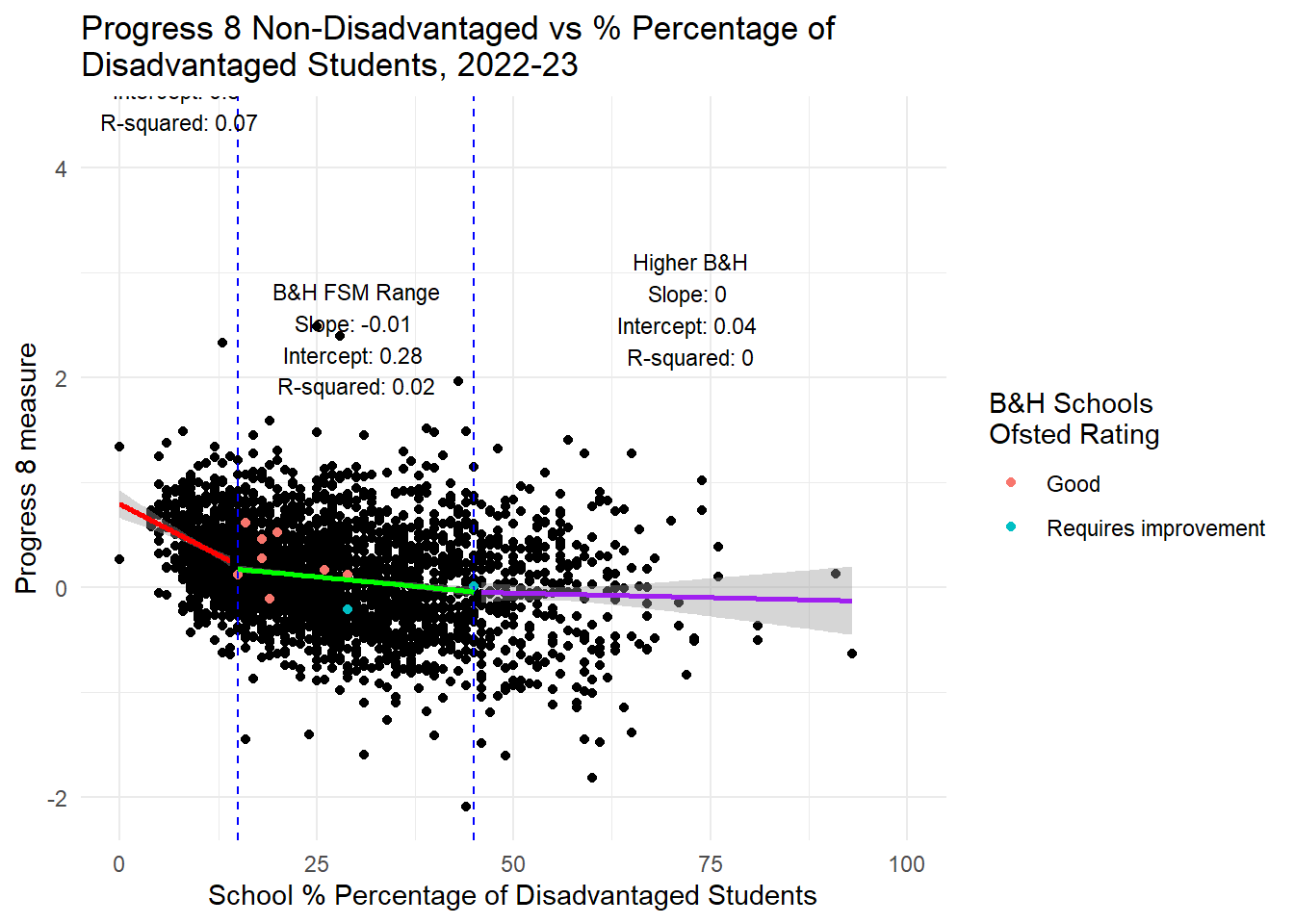

Progress Disadvantaged All

# Calculate the min and max values for the subset range
min_value <- min(btn_sub$PTFSM6CLA1A, na.rm = TRUE)
max_value <- max(btn_sub$PTFSM6CLA1A, na.rm = TRUE)

# Fit the linear model for the entire data
lm_model <- lm(P8MEA_FSM6CLA1A ~ PTFSM6CLA1A, data = england_school_2022_23_not_special)
lm_summary <- summary(lm_model)
slope <- lm_summary$coefficients[2, 1]
intercept <- lm_summary$coefficients[1, 1]
r_squared <- lm_summary$r.squared

# Annotation text
annotation_text <- paste("Slope:", round(slope, 2), "\nIntercept:", round(intercept, 2), "\nR-squared:", round(r_squared, 2))

# Plot the data with a linear regression line and annotation
ggplot(england_school_2022_23_not_special, aes(y = P8MEA_FSM6CLA1A, x = PTFSM6CLA1A)) +
  geom_point() +
  geom_point(data = btn_sub, aes(y = P8MEA_FSM6CLA1A, x = PTFSM6CLA1A, colour = OFSTEDRATING)) +
  geom_vline(xintercept = min_value, linetype = "dashed", color = "blue") +
  geom_vline(xintercept = max_value, linetype = "dashed", color = "blue") +
  geom_smooth(method = "lm", se = TRUE, color = "red") +
  labs(title = "Progress 8 Disadvantaged vs % School Percentage of \nDisadvantaged Students, 2022-23",
       x = "% Percentage of Disadvantaged Students",
       y = "Progress 8 measure",
       color = "B&H Schools \nOfsted Rating") +
  theme_minimal() +
  xlim(0, 100) +
  annotate("text", x = 80, y = min(england_school_2022_23_not_special$P8MEA_FSM6CLA1A, na.rm = TRUE), 
           label = annotation_text, hjust = 1, vjust = 0, size = 3)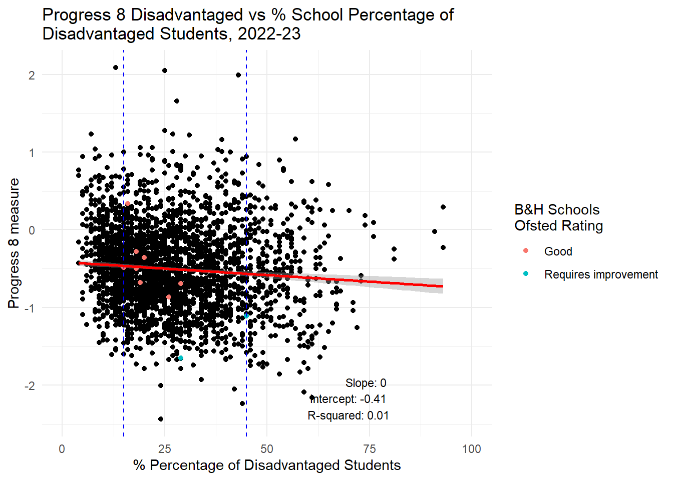

Progress Disadvantaged B&H Range

# Calculate the min and max values for the subset range
min_value <- min(btn_sub$PTFSM6CLA1A, na.rm = TRUE)
max_value <- max(btn_sub$PTFSM6CLA1A, na.rm = TRUE)

# Create the subset
subset_data <- england_school_2022_23_not_special %>%
  filter(PTFSM6CLA1A >= min_value & PTFSM6CLA1A <= max_value)

# Fit the linear model
lm_model <- lm(P8MEA_FSM6CLA1A ~ PTFSM6CLA1A, data = subset_data)
lm_summary <- summary(lm_model)
slope <- lm_summary$coefficients[2, 1]
intercept <- lm_summary$coefficients[1, 1]
r_squared <- lm_summary$r.squared

# Annotation text
annotation_text <- paste("Slope:", round(slope, 2), "\nIntercept:", round(intercept, 2), "\nR-squared:", round(r_squared, 2))

# Plot the data with a linear regression line and annotation
ggplot(subset_data, aes(y = P8MEA_FSM6CLA1A, x = PTFSM6CLA1A)) +
  geom_point() +
  geom_point(data = btn_sub, aes(y = P8MEA_FSM6CLA1A, x = PTFSM6CLA1A, colour = OFSTEDRATING)) +
  geom_vline(xintercept = min_value, linetype = "dashed", color = "blue") +
  geom_vline(xintercept = max_value, linetype = "dashed", color = "blue") +
  geom_smooth(method = "lm", se = TRUE, color = "red") +
  labs(title = "Progress 8 Disadvantaged vs % Percentage of \nDisadvantaged Students, 2022-23",
       x = "% Percentage of Disadvantaged Students",
       y = "Progress 8 measure",
       color = "B&H Schools \nOfsted Rating") +
  theme_minimal() +
  xlim(0, 100) +
  annotate("text", x = 80, y = min(subset_data$P8MEA_FSM6CLA1A, na.rm = TRUE), 
           label = annotation_text, hjust = 0.5, vjust = -1, size = 3)

Progress Disadvantaged Mixed Ranges

# Calculate the min and max values for the subset range
min_value <- min(btn_sub$PTFSM6CLA1A, na.rm = TRUE)
max_value <- max(btn_sub$PTFSM6CLA1A, na.rm = TRUE)

# Create subsets
subset_before <- england_school_2022_23_not_special %>%
  filter(PTFSM6CLA1A < min_value)

subset_after <- england_school_2022_23_not_special %>%
  filter(PTFSM6CLA1A > max_value)

subset_within <- england_school_2022_23_not_special %>%
  filter(PTFSM6CLA1A >= min_value & PTFSM6CLA1A <= max_value)

# Fit linear models
lm_before <- lm(P8MEA_FSM6CLA1A ~ PTFSM6CLA1A, data = subset_before)
lm_within <- lm(P8MEA_FSM6CLA1A ~ PTFSM6CLA1A, data = subset_within)
lm_after <- lm(P8MEA_FSM6CLA1A ~ PTFSM6CLA1A, data = subset_after)

# Calculate middle x positions for annotations
middle_before <- mean(c(0, min_value))
middle_within <- mean(c(min_value, max_value))
middle_after <- mean(c(max_value, 100))

# Plot the data with annotations
ggplot(england_school_2022_23_not_special, aes(y = P8MEA_FSM6CLA1A, x = PTFSM6CLA1A)) +
  geom_point() +
  geom_point(data = btn_sub, aes(y = P8MEA_FSM6CLA1A, x = PTFSM6CLA1A, colour = OFSTEDRATING)) +
  geom_vline(xintercept = min_value, linetype = "dashed", color = "blue") +
  geom_vline(xintercept = max_value, linetype = "dashed", color = "blue") +
  geom_smooth(data = subset_before, method = "lm", se = TRUE, color = "red", linetype = "solid", aes(group = 1)) +
  geom_smooth(data = subset_within, method = "lm", se = TRUE, color = "green", linetype = "solid", aes(group = 1)) +
  geom_smooth(data = subset_after, method = "lm", se = TRUE, color = "purple", linetype = "solid", aes(group = 1)) +
  labs(title = "Progress 8 Disadvantaged vs % Percentage of \nDisadvantaged Students, 2022-23",
       x = "School % Percentage of Disadvantaged Students",
       y = "Progress 8 measure",
       color = "B&H Schools \nOfsted Rating") +
  theme_minimal() +
  xlim(0, 100) +
  annotate("text", x = middle_before, y = min(subset_before$P8MEA_FSM6CLA1A, na.rm = TRUE) + 5, 
           label = paste("Lower B&H\nSlope:", round(coef(lm_before)[2], 2),
                         "\nIntercept:", round(coef(lm_before)[1], 2),
                         "\nR-squared:", round(summary(lm_before)$r.squared, 2)), 
           hjust = 0.5, vjust = 1, size = 3) +
  annotate("text", x = middle_within, y = min(subset_within$P8MEA_FSM6CLA1A, na.rm = TRUE) + 5, 
           label = paste("B&H FSM Range\nSlope:", round(coef(lm_within)[2], 2),
                         "\nIntercept:", round(coef(lm_within)[1], 2),
                         "\nR-squared:", round(summary(lm_within)$r.squared, 2)), 
           hjust = 0.5, vjust = 0.5, size = 3) +
  annotate("text", x = middle_after, y = min(subset_after$P8MEA_FSM6CLA1A, na.rm = TRUE) + 5, 
           label = paste("Higher B&H\nSlope:", round(coef(lm_after)[2], 2),
                         "\nIntercept:", round(coef(lm_after)[1], 2),
                         "\nR-squared:", round(summary(lm_after)$r.squared, 2)), 
           hjust = 0.5, vjust = 1, size = 3)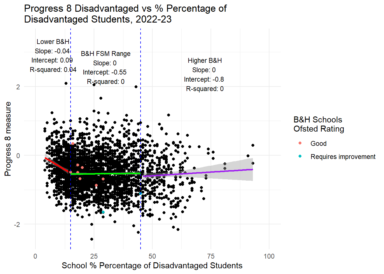

Persistent Absence

Attainment 8

Attainment Non-Disadvantaged All

# Calculate the min and max values for the subset range
min_value <- min(btn_sub$PPERSABS10, na.rm = TRUE)
max_value <- max(btn_sub$PPERSABS10, na.rm = TRUE)

# Fit the linear model for the entire data
lm_model <- lm(ATT8SCR_NFSM6CLA1A ~ PPERSABS10, data = england_school_2022_23_not_special)
lm_summary <- summary(lm_model)
slope <- lm_summary$coefficients[2, 1]
intercept <- lm_summary$coefficients[1, 1]
r_squared <- lm_summary$r.squared

# Annotation text
annotation_text <- paste("Slope:", round(slope, 2), "\nIntercept:", round(intercept, 2), "\nR-squared:", round(r_squared, 2))

# Plot the data with a linear regression line and annotation
ggplot(england_school_2022_23_not_special, aes(y = ATT8SCR_NFSM6CLA1A, x = PPERSABS10)) +
  geom_point() +
  geom_point(data = btn_sub, aes(y = ATT8SCR_NFSM6CLA1A, x = PPERSABS10, colour = OFSTEDRATING)) +
  geom_vline(xintercept = min_value, linetype = "dashed", color = "blue") +
  geom_vline(xintercept = max_value, linetype = "dashed", color = "blue") +
  geom_smooth(method = "lm", se = TRUE, color = "red") +
  labs(title = "Attainment 8 Non-Disadvantaged vs % School Percentage of \nPersistently Absent Students, 2022-23",
       x = "% Percentage of Persistently Absent Students",
       y = "Attainment 8 measure",
       color = "B&H Schools \nOfsted Rating") +
  theme_minimal() +
  xlim(0, 100) +
  annotate("text", x = 80, y = min(england_school_2022_23_not_special$ATT8SCR_NFSM6CLA1A, na.rm = TRUE), 
           label = annotation_text, hjust = 1, vjust = 0, size = 3)

Attainment Non-Disadvantaged B&H Range

# Calculate the min and max values for the subset range
min_value <- min(btn_sub$PPERSABS10, na.rm = TRUE)
max_value <- max(btn_sub$PPERSABS10, na.rm = TRUE)

# Create the subset
subset_data <- england_school_2022_23_not_special %>%
  filter(PPERSABS10 >= min_value & PPERSABS10 <= max_value)

# Fit the linear model
lm_model <- lm(ATT8SCR_NFSM6CLA1A ~ PPERSABS10, data = subset_data)
lm_summary <- summary(lm_model)
slope <- lm_summary$coefficients[2, 1]
intercept <- lm_summary$coefficients[1, 1]
r_squared <- lm_summary$r.squared

# Annotation text
annotation_text <- paste("Slope:", round(slope, 2), "\nIntercept:", round(intercept, 2), "\nR-squared:", round(r_squared, 2))

# Plot the data with a linear regression line and annotation
ggplot(subset_data, aes(y = ATT8SCR_NFSM6CLA1A, x = PPERSABS10)) +
  geom_point() +
  geom_point(data = btn_sub, aes(y = ATT8SCR_NFSM6CLA1A, x = PPERSABS10, colour = OFSTEDRATING)) +
  geom_vline(xintercept = min_value, linetype = "dashed", color = "blue") +
  geom_vline(xintercept = max_value, linetype = "dashed", color = "blue") +
  geom_smooth(method = "lm", se = TRUE, color = "red") +
  labs(title = "Attainment Non-Disadvantaged 8 vs % Percentage of \nPersistently Absent Students, 2022-23",
       x = "% Percentage of Persistently Absent Students",
       y = "Attainment 8 measure",
       color = "B&H Schools \nOfsted Rating") +
  theme_minimal() +
  xlim(0, 100) +
  annotate("text", x = 80, y = min(subset_data$ATT8SCR_NFSM6CLA1A, na.rm = TRUE), 
           label = annotation_text, hjust = 1, vjust = 0, size = 3)

Attainment Non-Disadvantaged Mixed Ranges

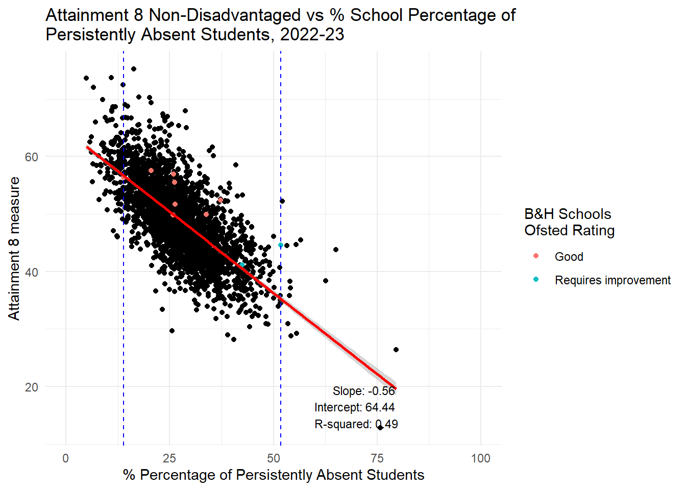
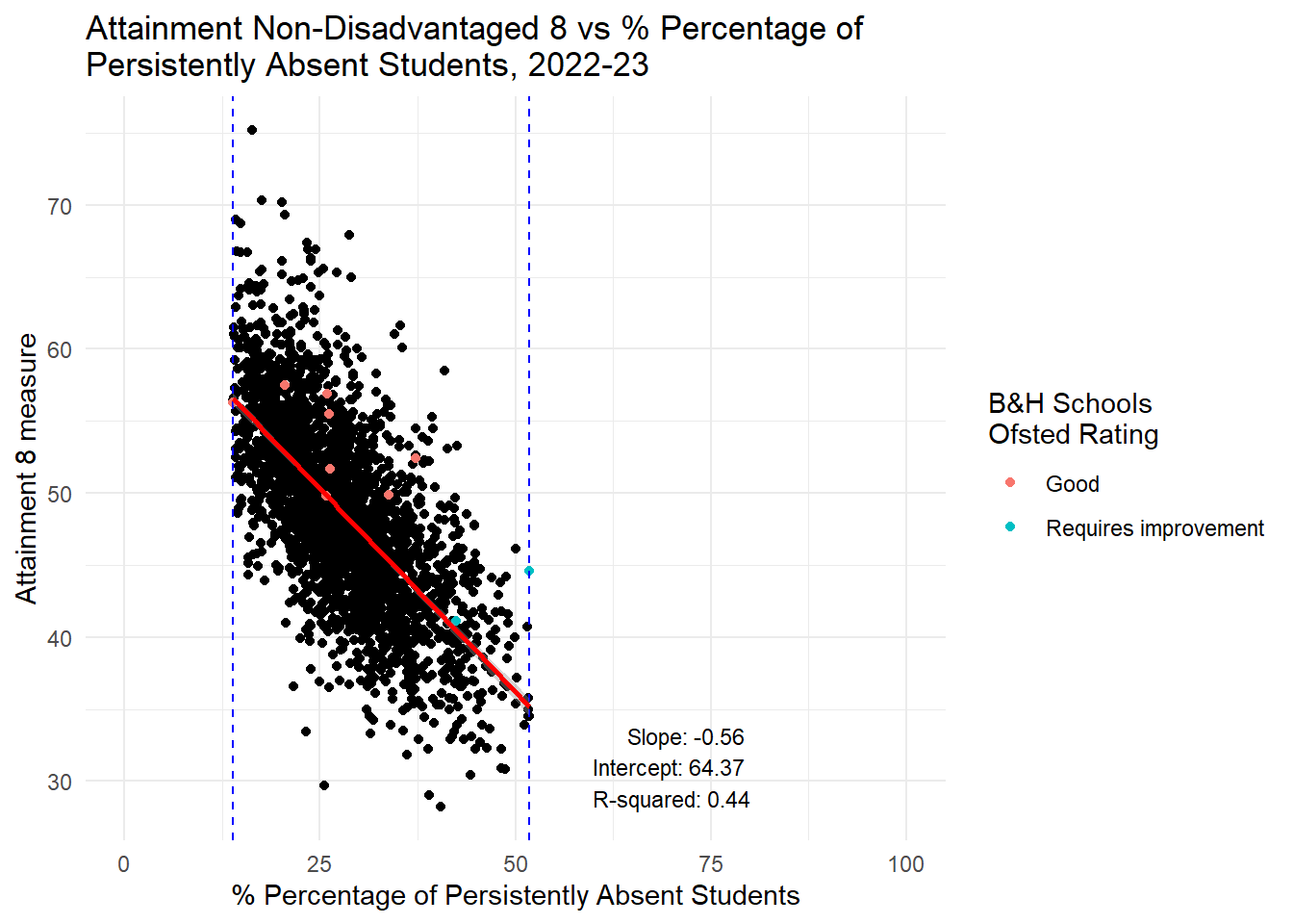
# Calculate the min and max values for the subset range
min_value <- min(btn_sub$PPERSABS10, na.rm = TRUE)
max_value <- max(btn_sub$PPERSABS10, na.rm = TRUE)

# Create subsets
subset_before <- england_school_2022_23_not_special %>%
  filter(PPERSABS10 < min_value)

subset_after <- england_school_2022_23_not_special %>%
  filter(PPERSABS10 > max_value)

subset_within <- england_school_2022_23_not_special %>%
  filter(PPERSABS10 >= min_value & PPERSABS10 <= max_value)

# Fit linear models
lm_before <- lm(ATT8SCR_NFSM6CLA1A ~ PPERSABS10, data = subset_before)
lm_within <- lm(ATT8SCR_NFSM6CLA1A ~ PPERSABS10, data = subset_within)
lm_after <- lm(ATT8SCR_NFSM6CLA1A ~ PPERSABS10, data = subset_after)

# Calculate middle x positions for annotations
middle_before <- mean(c(0, min_value))
middle_within <- mean(c(min_value, max_value))
middle_after <- mean(c(max_value, 100))

# Plot the data with annotations
ggplot(england_school_2022_23_not_special, aes(y = ATT8SCR_NFSM6CLA1A, x = PPERSABS10)) +
  geom_point() +
  geom_point(data = btn_sub, aes(y = ATT8SCR_NFSM6CLA1A, x = PPERSABS10, colour = OFSTEDRATING)) +
  geom_vline(xintercept = min_value, linetype = "dashed", color = "blue") +
  geom_vline(xintercept = max_value, linetype = "dashed", color = "blue") +
  geom_smooth(data = subset_before, method = "lm", se = TRUE, color = "red", linetype = "solid", aes(group = 1)) +
  geom_smooth(data = subset_within, method = "lm", se = TRUE, color = "green", linetype = "solid", aes(group = 1)) +
  geom_smooth(data = subset_after, method = "lm", se = TRUE, color = "purple", linetype = "solid", aes(group = 1)) +
  labs(title = "Attainment 8 Non-Disadvantaged vs % Percentage of \nPersistently Absent Students, 2022-23",
       x = "School % Percentage of Persistently Absent Students",
       y = "Attainment 8 measure",
       color = "B&H Schools \nOfsted Rating") +
  theme_minimal() +
  xlim(0, 100) +
  annotate("text", x = middle_before, y = min(subset_before$ATT8SCR_NFSM6CLA1A, na.rm = TRUE) + 5, 
           label = paste("Lower B&H\nSlope:", round(coef(lm_before)[2], 2),
                         "\nIntercept:", round(coef(lm_before)[1], 2),
                         "\nR-squared:", round(summary(lm_before)$r.squared, 2)), 
           hjust = 0.5, vjust = 0, size = 3) +
  annotate("text", x = middle_within, y = min(subset_within$ATT8SCR_NFSM6CLA1A, na.rm = TRUE) + 5, 
           label = paste("B&H P-Abs Range\nSlope:", round(coef(lm_within)[2], 2),
                         "\nIntercept:", round(coef(lm_within)[1], 2),
                         "\nR-squared:", round(summary(lm_within)$r.squared, 2)), 
           hjust = 0.5, vjust = 1, size = 3) +
  annotate("text", x = middle_after, y = min(subset_after$ATT8SCR_NFSM6CLA1A, na.rm = TRUE) + 5, 
           label = paste("Higher B&H\nSlope:", round(coef(lm_after)[2], 2),
                         "\nIntercept:", round(coef(lm_after)[1], 2),
                         "\nR-squared:", round(summary(lm_after)$r.squared, 2)), 
           hjust = 0.5, vjust = 1, size = 3)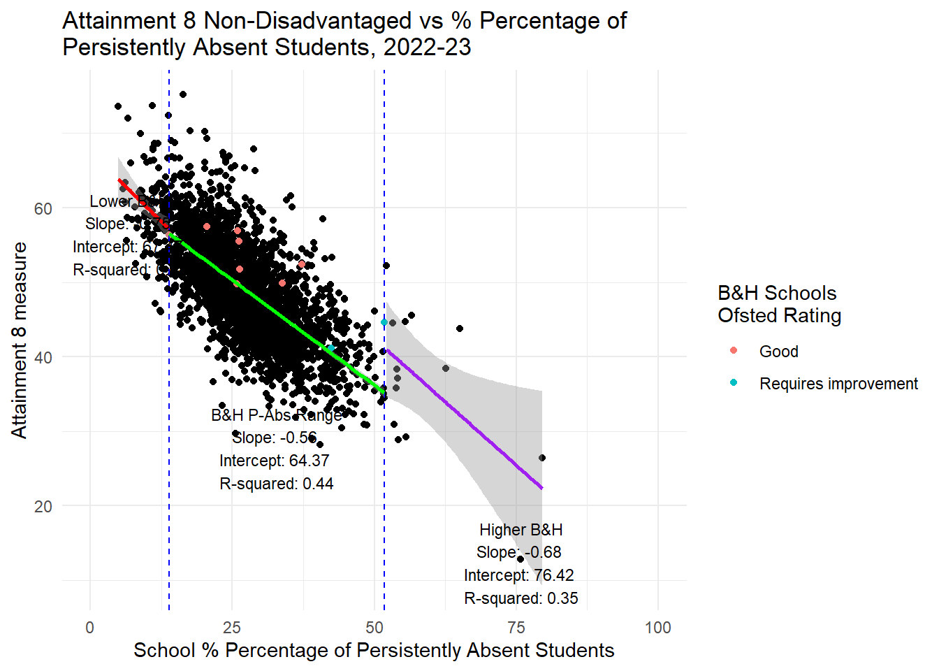

Attainment Disadvantaged All

# Calculate the min and max values for the subset range
min_value <- min(btn_sub$PPERSABS10, na.rm = TRUE)
max_value <- max(btn_sub$PPERSABS10, na.rm = TRUE)

# Fit the linear model for the entire data
lm_model <- lm(ATT8SCR_FSM6CLA1A ~ PPERSABS10, data = england_school_2022_23_not_special)
lm_summary <- summary(lm_model)
slope <- lm_summary$coefficients[2, 1]
intercept <- lm_summary$coefficients[1, 1]
r_squared <- lm_summary$r.squared

# Annotation text
annotation_text <- paste("Slope:", round(slope, 2), "\nIntercept:", round(intercept, 2), "\nR-squared:", round(r_squared, 2))

# Plot the data with a linear regression line and annotation
ggplot(england_school_2022_23_not_special, aes(y = ATT8SCR_FSM6CLA1A, x = PPERSABS10)) +
  geom_point() +
  geom_point(data = btn_sub, aes(y = ATT8SCR_FSM6CLA1A, x = PPERSABS10, colour = OFSTEDRATING)) +
  geom_vline(xintercept = min_value, linetype = "dashed", color = "blue") +
  geom_vline(xintercept = max_value, linetype = "dashed", color = "blue") +
  geom_smooth(method = "lm", se = TRUE, color = "red") +
  labs(title = "Attainment 8 Disadvantaged vs % School Percentage of \nPersistently Absent Students, 2022-23",
       x = "% Percentage of Persistently Absent Students",
       y = "Attainment 8 measure",
       color = "B&H Schools \nOfsted Rating") +
  theme_minimal() +
  xlim(0, 100) +
  annotate("text", x = 80, y = min(england_school_2022_23_not_special$ATT8SCR_FSM6CLA1A, na.rm = TRUE), 
           label = annotation_text, hjust = 1, vjust = 0, size = 3)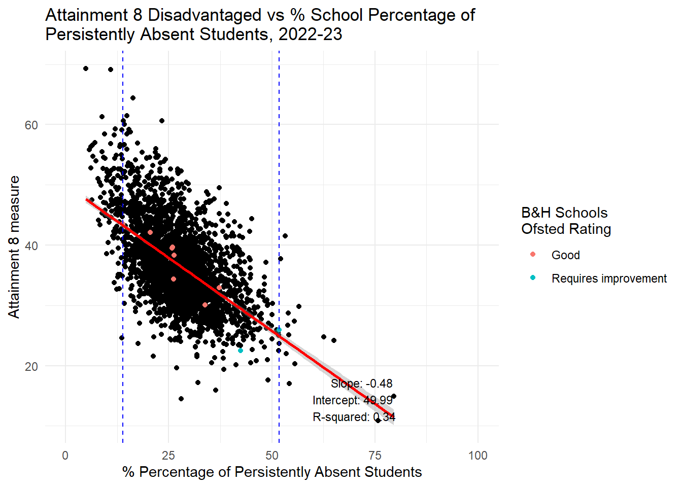

Attainment Disadvantaged B&H Range

# Calculate the min and max values for the subset range
min_value <- min(btn_sub$PPERSABS10, na.rm = TRUE)
max_value <- max(btn_sub$PPERSABS10, na.rm = TRUE)

# Create the subset
subset_data <- england_school_2022_23_not_special %>%
  filter(PPERSABS10 >= min_value & PPERSABS10 <= max_value)

# Fit the linear model
lm_model <- lm(ATT8SCR_FSM6CLA1A ~ PPERSABS10, data = subset_data)
lm_summary <- summary(lm_model)
slope <- lm_summary$coefficients[2, 1]
intercept <- lm_summary$coefficients[1, 1]
r_squared <- lm_summary$r.squared

# Annotation text
annotation_text <- paste("Slope:", round(slope, 2), "\nIntercept:", round(intercept, 2), "\nR-squared:", round(r_squared, 2))

# Plot the data with a linear regression line and annotation
ggplot(subset_data, aes(y = ATT8SCR_FSM6CLA1A, x = PPERSABS10)) +
  geom_point() +
  geom_point(data = btn_sub, aes(y = ATT8SCR_FSM6CLA1A, x = PPERSABS10, colour = OFSTEDRATING)) +
  geom_vline(xintercept = min_value, linetype = "dashed", color = "blue") +
  geom_vline(xintercept = max_value, linetype = "dashed", color = "blue") +
  geom_smooth(method = "lm", se = TRUE, color = "red") +
  labs(title = "Attainment Disadvantaged 8 vs % Percentage of \nPersistently Absent Students, 2022-23",
       x = "% Percentage of Persistently Absent Students",
       y = "Attainment 8 measure",
       color = "B&H Schools \nOfsted Rating") +
  theme_minimal() +
  xlim(0, 100) +
  annotate("text", x = 80, y = min(subset_data$ATT8SCR_FSM6CLA1A, na.rm = TRUE), 
           label = annotation_text, hjust = 1, vjust = 0, size = 3)

Attainment Disadvantaged Mixed Ranges

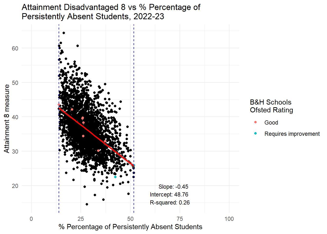
# Calculate the min and max values for the subset range
min_value <- min(btn_sub$PPERSABS10, na.rm = TRUE)
max_value <- max(btn_sub$PPERSABS10, na.rm = TRUE)

# Create subsets
subset_before <- england_school_2022_23_not_special %>%
  filter(PPERSABS10 < min_value)

subset_after <- england_school_2022_23_not_special %>%
  filter(PPERSABS10 > max_value)

subset_within <- england_school_2022_23_not_special %>%
  filter(PPERSABS10 >= min_value & PPERSABS10 <= max_value)

# Fit linear models
lm_before <- lm(ATT8SCR_FSM6CLA1A ~ PPERSABS10, data = subset_before)
lm_within <- lm(ATT8SCR_FSM6CLA1A ~ PPERSABS10, data = subset_within)
lm_after <- lm(ATT8SCR_FSM6CLA1A ~ PPERSABS10, data = subset_after)

# Calculate middle x positions for annotations
middle_before <- mean(c(0, min_value))
middle_within <- mean(c(min_value, max_value))
middle_after <- mean(c(max_value, 100))

# Plot the data with annotations
ggplot(england_school_2022_23_not_special, aes(y = ATT8SCR_FSM6CLA1A, x = PPERSABS10)) +
  geom_point() +
  geom_point(data = btn_sub, aes(y = ATT8SCR_FSM6CLA1A, x = PPERSABS10, colour = OFSTEDRATING)) +
  geom_vline(xintercept = min_value, linetype = "dashed", color = "blue") +
  geom_vline(xintercept = max_value, linetype = "dashed", color = "blue") +
  geom_smooth(data = subset_before, method = "lm", se = TRUE, color = "red", linetype = "solid", aes(group = 1)) +
  geom_smooth(data = subset_within, method = "lm", se = TRUE, color = "green", linetype = "solid", aes(group = 1)) +
  geom_smooth(data = subset_after, method = "lm", se = TRUE, color = "purple", linetype = "solid", aes(group = 1)) +
  labs(title = "Attainment 8 Disadvantaged vs % Percentage of \nPersistently Absent Students, 2022-23",
       x = "School % Percentage of Persistently Absent Students",
       y = "Attainment 8 measure",
       color = "B&H Schools \nOfsted Rating") +
  theme_minimal() +
  xlim(0, 100) +
  annotate("text", x = middle_before, y = min(subset_before$ATT8SCR_FSM6CLA1A, na.rm = TRUE) + 5, 
           label = paste("Lower B&H\nSlope:", round(coef(lm_before)[2], 2),
                         "\nIntercept:", round(coef(lm_before)[1], 2),
                         "\nR-squared:", round(summary(lm_before)$r.squared, 2)), 
           hjust = 0.5, vjust = 1, size = 3) +
  annotate("text", x = middle_within, y = min(subset_within$ATT8SCR_FSM6CLA1A, na.rm = TRUE) + 5, 
           label = paste("B&H P-Abs Range\nSlope:", round(coef(lm_within)[2], 2),
                         "\nIntercept:", round(coef(lm_within)[1], 2),
                         "\nR-squared:", round(summary(lm_within)$r.squared, 2)), 
           hjust = 0.5, vjust = -3, size = 3) +
  annotate("text", x = middle_after, y = min(subset_after$ATT8SCR_FSM6CLA1A, na.rm = TRUE) + 5, 
           label = paste("Higher B&H\nSlope:", round(coef(lm_after)[2], 2),
                         "\nIntercept:", round(coef(lm_after)[1], 2),
                         "\nR-squared:", round(summary(lm_after)$r.squared, 2)), 
           hjust = 0.5, vjust = -2.5, size = 3)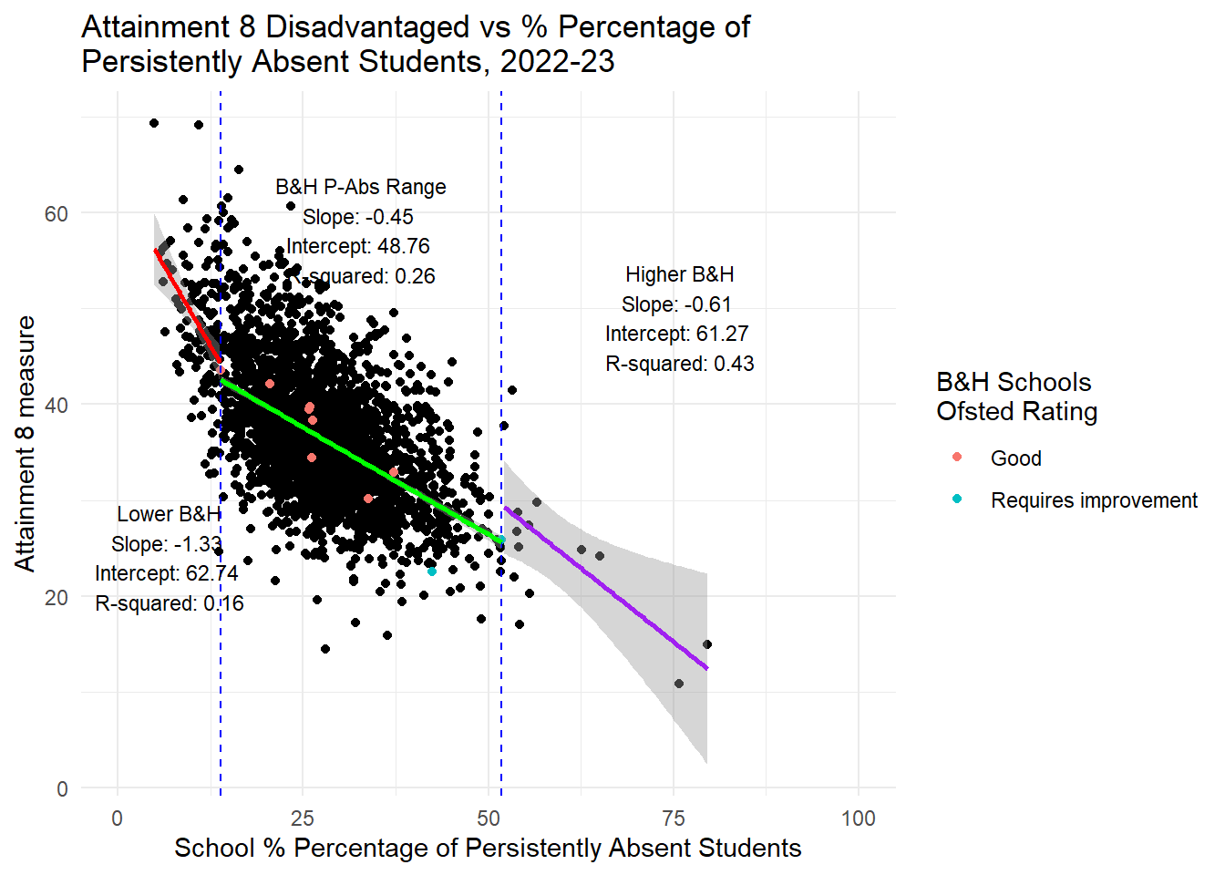

Progress 8

Progress Non-Disadvantaged All

# Calculate the min and max values for the subset range
min_value <- min(btn_sub$PPERSABS10, na.rm = TRUE)
max_value <- max(btn_sub$PPERSABS10, na.rm = TRUE)

# Fit the linear model for the entire data
lm_model <- lm(P8MEA_NFSM6CLA1A ~ PPERSABS10, data = england_school_2022_23_not_special)
lm_summary <- summary(lm_model)
slope <- lm_summary$coefficients[2, 1]
intercept <- lm_summary$coefficients[1, 1]
r_squared <- lm_summary$r.squared

# Annotation text
annotation_text <- paste("Slope:", round(slope, 2), "\nIntercept:", round(intercept, 2), "\nR-squared:", round(r_squared, 2))

# Plot the data with a linear regression line and annotation
ggplot(england_school_2022_23_not_special, aes(y = P8MEA_NFSM6CLA1A, x = PPERSABS10)) +
  geom_point() +
  geom_point(data = btn_sub, aes(y = P8MEA_NFSM6CLA1A, x = PPERSABS10, colour = OFSTEDRATING)) +
  geom_vline(xintercept = min_value, linetype = "dashed", color = "blue") +
  geom_vline(xintercept = max_value, linetype = "dashed", color = "blue") +
  geom_smooth(method = "lm", se = TRUE, color = "red") +
  labs(title = "Progress 8 Non-Disadvantaged vs % School Percentage of \nPersistently Absent Students, 2022-23",
       x = "% Percentage of Persistently Absent Students",
       y = "Progress 8 measure",
       color = "B&H Schools \nOfsted Rating") +
  theme_minimal() +
  xlim(0, 100) +
  annotate("text", x = 80, y = min(england_school_2022_23_not_special$P8MEA_NFSM6CLA1A, na.rm = TRUE), 
           label = annotation_text, hjust = 1, vjust = 0, size = 3)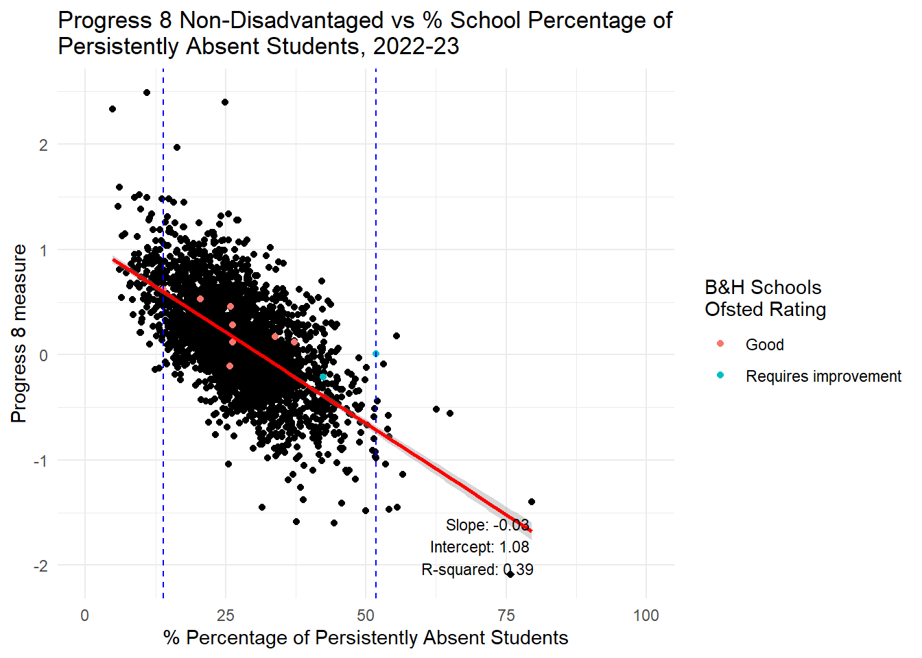

Progress Non-Disadvantaged B&H Range

# Calculate the min and max values for the subset range
min_value <- min(btn_sub$PPERSABS10, na.rm = TRUE)
max_value <- max(btn_sub$PPERSABS10, na.rm = TRUE)

# Create the subset
subset_data <- england_school_2022_23_not_special %>%
  filter(PPERSABS10 >= min_value & PPERSABS10 <= max_value)

# Fit the linear model
lm_model <- lm(P8MEA_NFSM6CLA1A ~ PPERSABS10, data = subset_data)
lm_summary <- summary(lm_model)
slope <- lm_summary$coefficients[2, 1]
intercept <- lm_summary$coefficients[1, 1]
r_squared <- lm_summary$r.squared

# Annotation text
annotation_text <- paste("Slope:", round(slope, 2), "\nIntercept:", round(intercept, 2), "\nR-squared:", round(r_squared, 2))

# Plot the data with a linear regression line and annotation
ggplot(subset_data, aes(y = P8MEA_NFSM6CLA1A, x = PPERSABS10)) +
  geom_point() +
  geom_point(data = btn_sub, aes(y = P8MEA_NFSM6CLA1A, x = PPERSABS10, colour = OFSTEDRATING)) +
  geom_vline(xintercept = min_value, linetype = "dashed", color = "blue") +
  geom_vline(xintercept = max_value, linetype = "dashed", color = "blue") +
  geom_smooth(method = "lm", se = TRUE, color = "red") +
  labs(title = "Progress 8 Non-Disadvantaged vs % Percentage of \nPersistently Absent Students, 2022-23",
       x = "% Percentage of Persistently Absent Students",
       y = "Progress 8 measure",
       color = "B&H Schools \nOfsted Rating") +
  theme_minimal() +
  xlim(0, 100) +
  annotate("text", x = 80, y = min(subset_data$P8MEA_NFSM6CLA1A, na.rm = TRUE), 
           label = annotation_text, hjust = 1, vjust = 0, size = 3)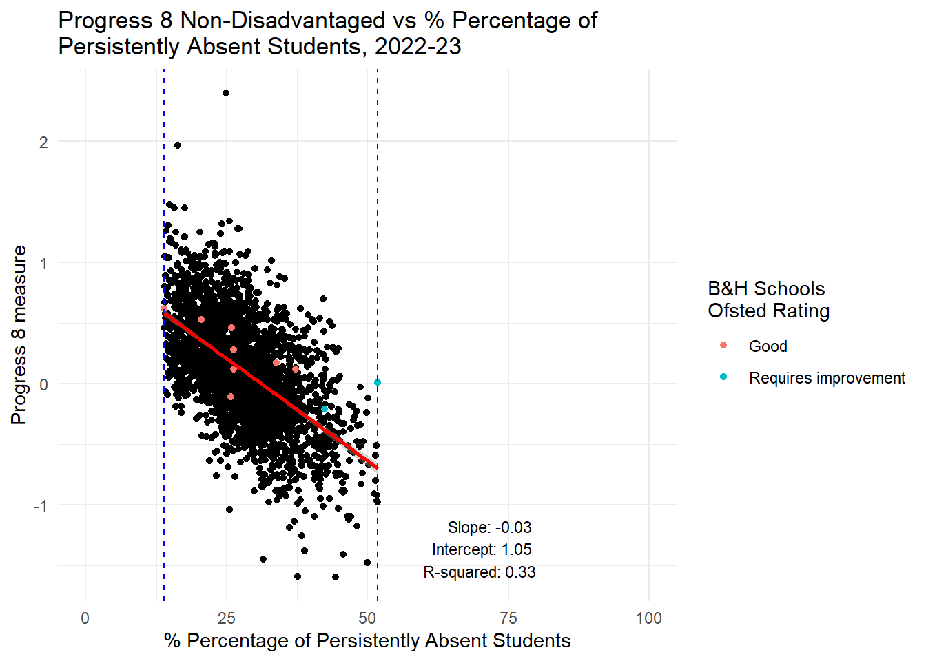

Progress Non-Disadvantaged Mixed Ranges

# Calculate the min and max values for the subset range
min_value <- min(btn_sub$PPERSABS10, na.rm = TRUE)
max_value <- max(btn_sub$PPERSABS10, na.rm = TRUE)

# Create subsets
subset_before <- england_school_2022_23_not_special %>%
  filter(PPERSABS10 < min_value)

subset_after <- england_school_2022_23_not_special %>%
  filter(PPERSABS10 > max_value)

subset_within <- england_school_2022_23_not_special %>%
  filter(PPERSABS10 >= min_value & PPERSABS10 <= max_value)

# Fit linear models
lm_before <- lm(P8MEA_NFSM6CLA1A ~ PPERSABS10, data = subset_before)
lm_within <- lm(P8MEA_NFSM6CLA1A ~ PPERSABS10, data = subset_within)
lm_after <- lm(P8MEA_NFSM6CLA1A ~ PPERSABS10, data = subset_after)

# Calculate middle x positions for annotations
middle_before <- mean(c(0, min_value))
middle_within <- mean(c(min_value, max_value))
middle_after <- mean(c(max_value, 100))

# Plot the data with annotations
ggplot(england_school_2022_23_not_special, aes(y = P8MEA_NFSM6CLA1A, x = PPERSABS10)) +
  geom_point() +
  geom_point(data = btn_sub, aes(y = P8MEA_NFSM6CLA1A, x = PPERSABS10, colour = OFSTEDRATING)) +
  geom_vline(xintercept = min_value, linetype = "dashed", color = "blue") +
  geom_vline(xintercept = max_value, linetype = "dashed", color = "blue") +
  geom_smooth(data = subset_before, method = "lm", se = TRUE, color = "red", linetype = "solid", aes(group = 1)) +
  geom_smooth(data = subset_within, method = "lm", se = TRUE, color = "green", linetype = "solid", aes(group = 1)) +
  geom_smooth(data = subset_after, method = "lm", se = TRUE, color = "purple", linetype = "solid", aes(group = 1)) +
  labs(title = "Progress 8 Non-Disadvantaged vs % Percentage of \nPersistently Absent Students, 2022-23",
       x = "School % Percentage of Persistently Absent Students",
       y = "Progress 8 measure",
       color = "B&H Schools \nOfsted Rating") +
  theme_minimal() +
  xlim(0, 100) +
  annotate("text", x = middle_before, y = min(subset_before$P8MEA_NFSM6CLA1A, na.rm = TRUE) + 5, 
           label = paste("Lower B&H\nSlope:", round(coef(lm_before)[2], 2),
                         "\nIntercept:", round(coef(lm_before)[1], 2),
                         "\nR-squared:", round(summary(lm_before)$r.squared, 2)), 
           hjust = 0.5, vjust = 1, size = 3) +
  annotate("text", x = middle_within, y = min(subset_within$P8MEA_NFSM6CLA1A, na.rm = TRUE) + 5, 
           label = paste("B&H P-Abs Range\nSlope:", round(coef(lm_within)[2], 2),
                         "\nIntercept:", round(coef(lm_within)[1], 2),
                         "\nR-squared:", round(summary(lm_within)$r.squared, 2)), 
           hjust = 0.5, vjust = 1, size = 3) +
  annotate("text", x = middle_after, y = min(subset_after$P8MEA_NFSM6CLA1A, na.rm = TRUE) + 5, 
           label = paste("Higher B&H\nSlope:", round(coef(lm_after)[2], 2),
                         "\nIntercept:", round(coef(lm_after)[1], 2),
                         "\nR-squared:", round(summary(lm_after)$r.squared, 2)), 
           hjust = 0.5, vjust = 1, size = 3)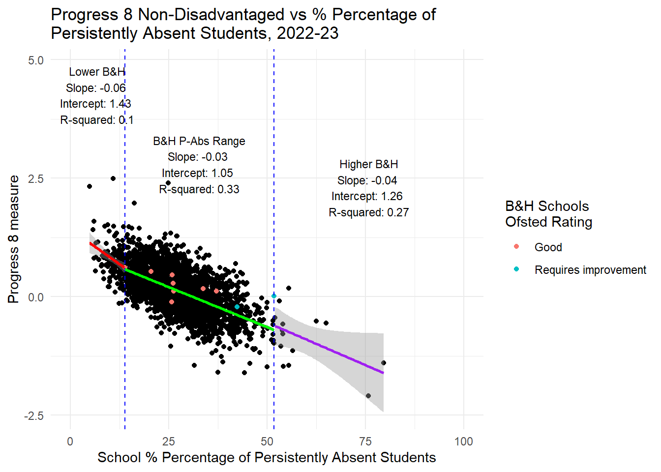

Progress Disadvantaged All

# Calculate the min and max values for the subset range
min_value <- min(btn_sub$PPERSABS10, na.rm = TRUE)
max_value <- max(btn_sub$PPERSABS10, na.rm = TRUE)

# Fit the linear model for the entire data
lm_model <- lm(P8MEA_FSM6CLA1A ~ PPERSABS10, data = england_school_2022_23_not_special)
lm_summary <- summary(lm_model)
slope <- lm_summary$coefficients[2, 1]
intercept <- lm_summary$coefficients[1, 1]
r_squared <- lm_summary$r.squared

# Annotation text
annotation_text <- paste("Slope:", round(slope, 2), "\nIntercept:", round(intercept, 2), "\nR-squared:", round(r_squared, 2))

# Plot the data with a linear regression line and annotation
ggplot(england_school_2022_23_not_special, aes(y = P8MEA_FSM6CLA1A, x = PPERSABS10)) +
  geom_point() +
  geom_point(data = btn_sub, aes(y = P8MEA_FSM6CLA1A, x = PPERSABS10, colour = OFSTEDRATING)) +
  geom_vline(xintercept = min_value, linetype = "dashed", color = "blue") +
  geom_vline(xintercept = max_value, linetype = "dashed", color = "blue") +
  geom_smooth(method = "lm", se = TRUE, color = "red") +
  labs(title = "Progress 8 Disadvantaged vs % School Percentage of \nPersistently Absent Students, 2022-23",
       x = "% Percentage of Persistently Absent Students",
       y = "Progress 8 measure",
       color = "B&H Schools \nOfsted Rating") +
  theme_minimal() +
  xlim(0, 100) +
  annotate("text", x = 80, y = min(england_school_2022_23_not_special$P8MEA_FSM6CLA1A, na.rm = TRUE), 
           label = annotation_text, hjust = 1, vjust = 0, size = 3)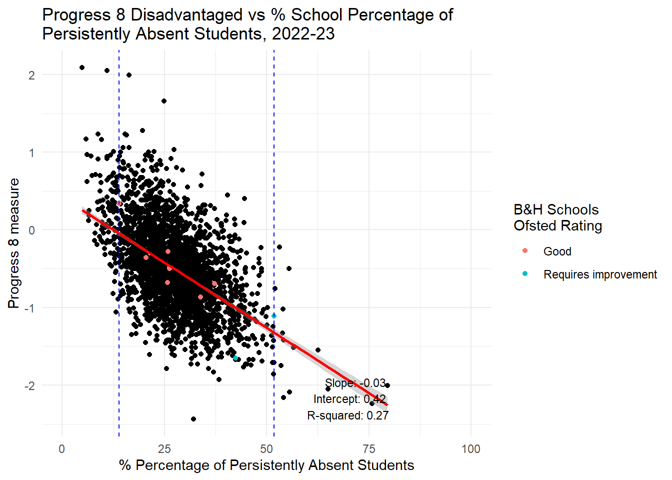

Progress Disadvantaged B&H Range

# Calculate the min and max values for the subset range
min_value <- min(btn_sub$PPERSABS10, na.rm = TRUE)
max_value <- max(btn_sub$PPERSABS10, na.rm = TRUE)

# Create the subset
subset_data <- england_school_2022_23_not_special %>%
  filter(PPERSABS10 >= min_value & PPERSABS10 <= max_value)

# Fit the linear model
lm_model <- lm(P8MEA_FSM6CLA1A ~ PPERSABS10, data = subset_data)
lm_summary <- summary(lm_model)
slope <- lm_summary$coefficients[2, 1]
intercept <- lm_summary$coefficients[1, 1]
r_squared <- lm_summary$r.squared

# Annotation text
annotation_text <- paste("Slope:", round(slope, 2), "\nIntercept:", round(intercept, 2), "\nR-squared:", round(r_squared, 2))

# Plot the data with a linear regression line and annotation
ggplot(subset_data, aes(y = P8MEA_FSM6CLA1A, x = PPERSABS10)) +
  geom_point() +
  geom_point(data = btn_sub, aes(y = P8MEA_FSM6CLA1A, x = PPERSABS10, colour = OFSTEDRATING)) +
  geom_vline(xintercept = min_value, linetype = "dashed", color = "blue") +
  geom_vline(xintercept = max_value, linetype = "dashed", color = "blue") +
  geom_smooth(method = "lm", se = TRUE, color = "red") +
  labs(title = "Progress 8 Disadvantaged vs % Percentage of \nPersistently Absent Students, 2022-23",
       x = "% Percentage of Persistently Absent Students",
       y = "Progress 8 measure",
       color = "B&H Schools \nOfsted Rating") +
  theme_minimal() +
  xlim(0, 100) +
  annotate("text", x = 80, y = min(subset_data$P8MEA_FSM6CLA1A, na.rm = TRUE), 
           label = annotation_text, hjust = 0.5, vjust = -1, size = 3)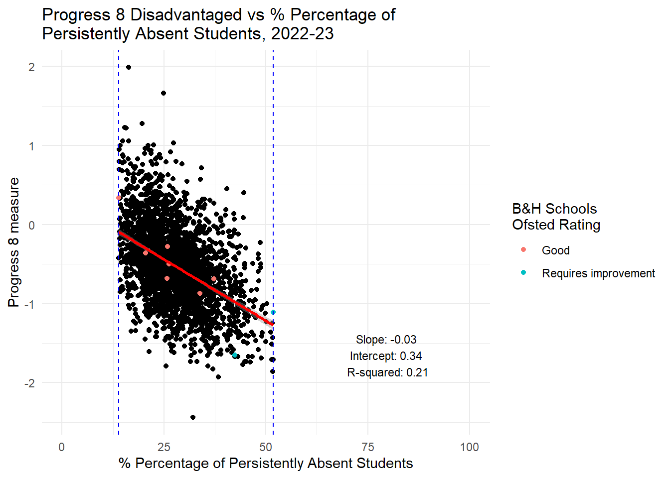

Progress Disadvantaged Mixed Ranges

# Calculate the min and max values for the subset range
min_value <- min(btn_sub$PPERSABS10, na.rm = TRUE)
max_value <- max(btn_sub$PPERSABS10, na.rm = TRUE)

# Create subsets
subset_before <- england_school_2022_23_not_special %>%
  filter(PPERSABS10 < min_value)

subset_after <- england_school_2022_23_not_special %>%
  filter(PPERSABS10 > max_value)

subset_within <- england_school_2022_23_not_special %>%
  filter(PPERSABS10 >= min_value & PPERSABS10 <= max_value)

# Fit linear models
lm_before <- lm(P8MEA_FSM6CLA1A ~ PPERSABS10, data = subset_before)
lm_within <- lm(P8MEA_FSM6CLA1A ~ PPERSABS10, data = subset_within)
lm_after <- lm(P8MEA_FSM6CLA1A ~ PPERSABS10, data = subset_after)

# Calculate middle x positions for annotations
middle_before <- mean(c(0, min_value))
middle_within <- mean(c(min_value, max_value))
middle_after <- mean(c(max_value, 100))

# Plot the data with annotations
ggplot(england_school_2022_23_not_special, aes(y = P8MEA_FSM6CLA1A, x = PPERSABS10)) +
  geom_point() +
  geom_point(data = btn_sub, aes(y = P8MEA_FSM6CLA1A, x = PPERSABS10, colour = OFSTEDRATING)) +
  geom_vline(xintercept = min_value, linetype = "dashed", color = "blue") +
  geom_vline(xintercept = max_value, linetype = "dashed", color = "blue") +
  geom_smooth(data = subset_before, method = "lm", se = TRUE, color = "red", linetype = "solid", aes(group = 1)) +
  geom_smooth(data = subset_within, method = "lm", se = TRUE, color = "green", linetype = "solid", aes(group = 1)) +
  geom_smooth(data = subset_after, method = "lm", se = TRUE, color = "purple", linetype = "solid", aes(group = 1)) +
  labs(title = "Progress 8 Disadvantaged vs % Percentage of \nPersistently Absent Students, 2022-23",
       x = "School % Percentage of Persistently Absent Students",
       y = "Progress 8 measure",
       color = "B&H Schools \nOfsted Rating") +
  theme_minimal() +
  xlim(0, 100) +
  annotate("text", x = middle_before, y = min(subset_before$P8MEA_FSM6CLA1A, na.rm = TRUE) + 5, 
           label = paste("Lower B&H\nSlope:", round(coef(lm_before)[2], 2),
                         "\nIntercept:", round(coef(lm_before)[1], 2),
                         "\nR-squared:", round(summary(lm_before)$r.squared, 2)), 
           hjust = 0.5, vjust = 1, size = 3) +
  annotate("text", x = middle_within, y = min(subset_within$P8MEA_FSM6CLA1A, na.rm = TRUE) + 5, 
           label = paste("B&H P-Abs Range\nSlope:", round(coef(lm_within)[2], 2),
                         "\nIntercept:", round(coef(lm_within)[1], 2),
                         "\nR-squared:", round(summary(lm_within)$r.squared, 2)), 
           hjust = 0.5, vjust = 0.5, size = 3) +
  annotate("text", x = middle_after, y = min(subset_after$P8MEA_FSM6CLA1A, na.rm = TRUE) + 5, 
           label = paste("Higher B&H\nSlope:", round(coef(lm_after)[2], 2),
                         "\nIntercept:", round(coef(lm_after)[1], 2),
                         "\nR-squared:", round(summary(lm_after)$r.squared, 2)), 
           hjust = 0.5, vjust = 1, size = 3)