Show code
library(readxl)
library(sf)
library(dplyr)
library(tidyr)
library(readr)
library(leaflet)
library(tmap)
library(classInt)
library(htmltools)
library(knitr)
library(kableExtra)
library(jsonlite)
library(ggplot2)This analysis compares the current provision of 24/7 publicly accessible Automated External Defibrillators (AEDs) in Brighton & Hove against two complementary measures of population demand:
By examining both perspectives, we can identify areas with high demand but low defibrillator coverage and understand how priority rankings shift depending on whether we consider daytime or residential populations.
Data sources:
library(readxl)
library(sf)
library(dplyr)
library(tidyr)
library(readr)
library(leaflet)
library(tmap)
library(classInt)
library(htmltools)
library(knitr)
library(kableExtra)
library(jsonlite)
library(ggplot2)# Load full dataset
defib <- read_excel("defibrillator_data.xlsx",
sheet = "data_extract_2026-02-02")
# Filter to Brighton & Hove
bh_defib <- defib %>%
filter(grepl("Brighton", ladnm, ignore.case = TRUE),
!is.na(lat), !is.na(long))
cat("Total AEDs in Brighton & Hove:", nrow(bh_defib), "\n")Total AEDs in Brighton & Hove: 275 # Summary by availability and access type
bh_defib %>%
count(defibrillators_availability, defibrillators_access_type,
name = "count") %>%
arrange(desc(count)) %>%
kable(col.names = c("Availability", "Access Type", "Count")) %>%
kable_styling(bootstrap_options = c("striped", "hover"), full_width = FALSE)| Availability | Access Type | Count |
|---|---|---|
| 24/7 Access | Public | 108 |
| Varied Access | Restricted | 96 |
| Varied Access | Public | 62 |
| 24/7 Access | Restricted | 9 |
# Filter to 24/7 public access defibrillators only
bh_247_public <- bh_defib %>%
  filter(defibrillators_availability == "24/7 Access",
         defibrillators_access_type == "Public")

cat("24/7 Public AEDs in Brighton & Hove:", nrow(bh_247_public), "\n")
24/7 Public AEDs in Brighton & Hove: 108 # Convert to spatial
bh_247_sf <- st_as_sf(bh_247_public, coords = c("long", "lat"), crs = 4326)
# Also create sf for ALL B&H defibrillators (for context)
bh_all_sf <- st_as_sf(bh_defib, coords = c("long", "lat"), crs = 4326)# Download Brighton & Hove LSOA boundaries from ONS ArcGIS FeatureServer
# Using the BGC (Generalised Clipped) V5 version for higher-quality boundaries
api_url <- paste0(
"https://services1.arcgis.com/ESMARspQHYMw9BZ9/arcgis/rest/services/",
"Lower_layer_Super_Output_Areas_December_2021_Boundaries_EW_BGC_V5/",
"FeatureServer/0/query?",
"where=LSOA21NM+LIKE+%27Brighton%25%27",
"&outFields=LSOA21CD,LSOA21NM",
"&returnGeometry=true",
"&outSR=4326",
"&f=geojson",
"&resultRecordCount=200"
)
# Download to temp file and read
tmp_geojson <- tempfile(fileext = ".geojson")
download.file(api_url, tmp_geojson, quiet = TRUE, mode = "wb")
bh_lsoa <- st_read(tmp_geojson, quiet = TRUE)
cat("LSOA boundaries loaded:", nrow(bh_lsoa), "LSOAs\n")LSOA boundaries loaded: 165 LSOAs# Download WD001 from Nomis
tmp_zip <- tempfile(fileext = ".zip")
download.file("https://www.nomisweb.co.uk/output/census/2021/wd001.zip",
tmp_zip, quiet = TRUE, mode = "wb")
# Extract and read the LSOA-level CSV
tmp_dir <- tempdir()
unzip(tmp_zip, exdir = tmp_dir)
wd001 <- read_csv(file.path(tmp_dir, "WD001_lsoa.csv"),
show_col_types = FALSE)
# Rename columns for easier use
wd001 <- wd001 %>%
rename(
lsoa21cd = `Lower layer Super Output Areas Code`,
lsoa21nm = `Lower layer Super Output Areas Label`,
workday_density = `Population Density`
)
# Filter to Brighton & Hove LSOAs
bh_wd001 <- wd001 %>%
filter(lsoa21cd %in% bh_lsoa$LSOA21CD)
cat("Workday density data for", nrow(bh_wd001), "Brighton & Hove LSOAs\n")Workday density data for 165 Brighton & Hove LSOAscat("Range:", round(min(bh_wd001$workday_density)),
"to", round(max(bh_wd001$workday_density)),
"persons per km²\n")Range: 267 to 52028 persons per km²# Download TS001 (usual resident population) from Nomis Census 2021 bulk data
tmp_zip_ts <- tempfile(fileext = ".zip")
download.file("https://www.nomisweb.co.uk/output/census/2021/census2021-ts001.zip",
tmp_zip_ts, quiet = TRUE, mode = "wb")
# Extract to a dedicated subdirectory to avoid file conflicts
tmp_dir_ts <- file.path(tempdir(), "ts001")
dir.create(tmp_dir_ts, showWarnings = FALSE)
unzip(tmp_zip_ts, exdir = tmp_dir_ts)
# Find the LSOA-level CSV
ts_files <- list.files(tmp_dir_ts, pattern = "\\.csv$",
full.names = TRUE, recursive = TRUE)
ts001_file <- ts_files[grep("lsoa", ts_files, ignore.case = TRUE)][1]
ts001_raw <- read_csv(ts001_file, show_col_types = FALSE)
# Identify columns flexibly (Census 2021 bulk CSVs vary in naming)
code_col <- names(ts001_raw)[grep("geography.code|Areas.Code|LSOA.*Code",
names(ts001_raw), ignore.case = TRUE)][1]
total_col <- names(ts001_raw)[grep("Total|Usual.resident",
names(ts001_raw), ignore.case = TRUE)][1]
bh_ts001 <- ts001_raw %>%
select(lsoa21cd = all_of(code_col),
resident_pop = all_of(total_col)) %>%
filter(lsoa21cd %in% bh_lsoa$LSOA21CD)
cat("Resident population data for", nrow(bh_ts001), "Brighton & Hove LSOAs\n")Resident population data for 165 Brighton & Hove LSOAscat("Total usual residents:", format(sum(bh_ts001$resident_pop), big.mark = ","), "\n")Total usual residents: 277,095 Telephone boxes are potential sites for new defibrillator installations — many across the UK have already been converted. We download current telephone box locations from OpenStreetMap via the Overpass API (amenity=telephone).
# Query OSM Overpass API for telephone boxes in Brighton & Hove
# Use a bounding box around Brighton & Hove to avoid URL encoding issues
# with area names. B&H bbox: south=50.79, west=-0.30, north=50.89, east=-0.04
overpass_query <- '[out:json][timeout:30];node[amenity=telephone](50.79,-0.30,50.89,-0.04);out body;'
overpass_url <- paste0(
  "https://overpass-api.de/api/interpreter?data=",
  URLencode(overpass_query, reserved = TRUE)
)

osm_raw <- fromJSON(overpass_url)

phone_boxes <- osm_raw$elements %>%
  select(id, lat, lon) %>%
  filter(!is.na(lat), !is.na(lon))

phone_sf <- st_as_sf(phone_boxes, coords = c("lon", "lat"), crs = 4326)

cat("Telephone boxes loaded from OSM:", nrow(phone_sf), "\n")
Telephone boxes loaded from OSM: 56 # Count 24/7 public AEDs per LSOA
aed_counts <- bh_247_public %>%
count(lsoa21, name = "aed_count")
# Join workday density to LSOA boundaries
bh_analysis <- bh_lsoa %>%
left_join(bh_wd001, by = c("LSOA21CD" = "lsoa21cd")) %>%
left_join(aed_counts, by = c("LSOA21CD" = "lsoa21")) %>%
mutate(
aed_count = replace_na(aed_count, 0),
# Priority score: higher workday density with fewer AEDs = higher priority
priority_score = workday_density / (aed_count + 1),
priority_rank = rank(-priority_score, ties.method = "first")
)
cat("LSOAs with zero 24/7 public AEDs:",
sum(bh_analysis$aed_count == 0), "of", nrow(bh_analysis), "\n")LSOAs with zero 24/7 public AEDs: 102 of 165 This map shows the Census 2021 workday population density across Brighton & Hove LSOAs. Darker shading indicates higher concentrations of people during the working day. Red points show the locations of existing 24/7 publicly accessible defibrillators.
tmap_mode("plot")

tm_shape(bh_analysis) +
  tm_polygons(
    fill = "workday_density",
    fill.scale = tm_scale_continuous(
      values = "brewer.blues"
    ),
    fill.legend = tm_legend(
      title = "Workday Pop.\nDensity\n(per km²)"
    ),
    col = "grey60",
    lwd = 0.5
  ) +
  tm_shape(bh_247_sf) +
  tm_symbols(
    fill = "red",
    col = "darkred",
    size = 0.3,
    shape = 21
  ) +
  tm_title("Workday Population Demand & 24/7 Public AED Locations") +
  tm_layout(
    frame = FALSE
  ) +
  tm_scalebar(position = c("left", "bottom"))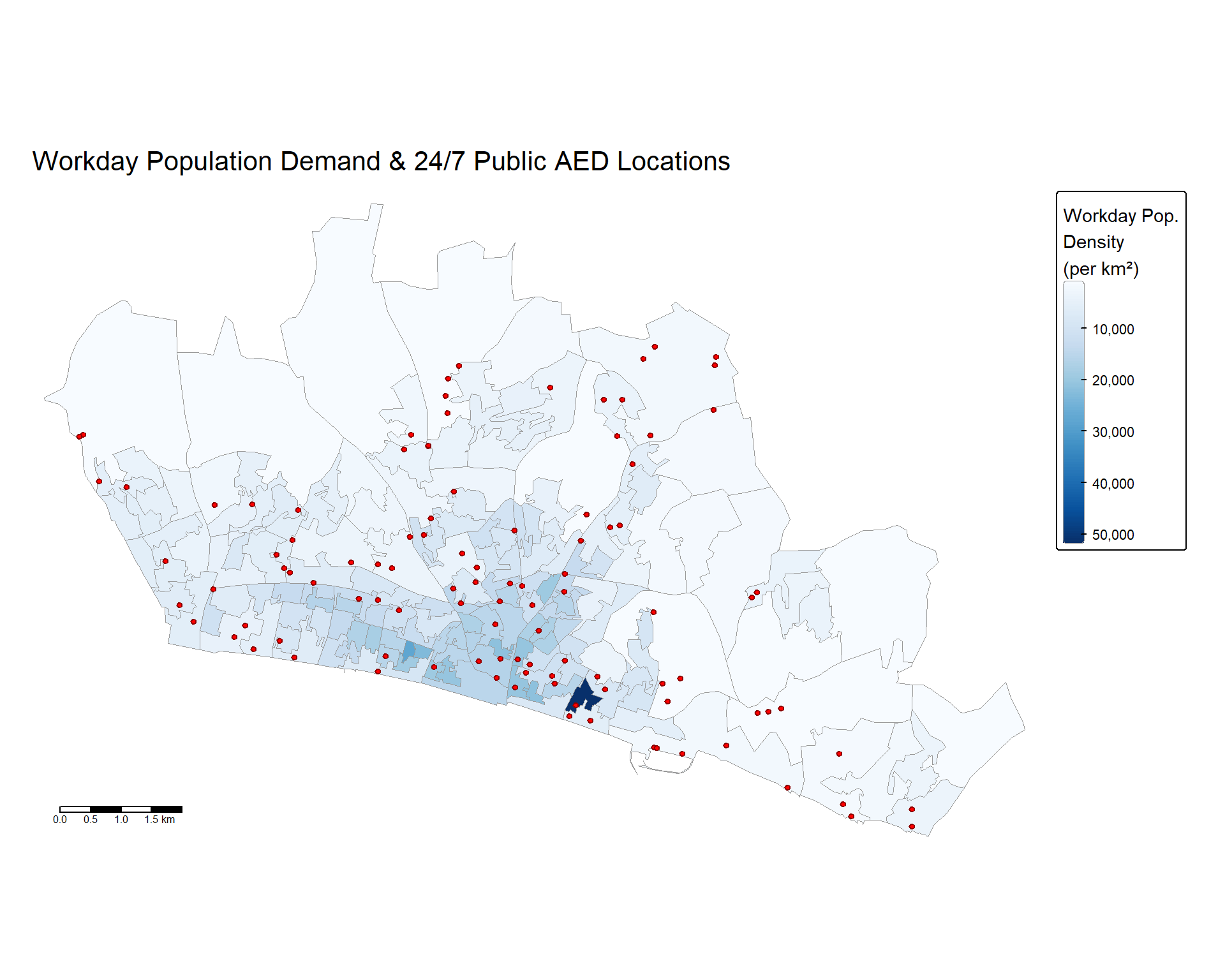
Zoom in to explore individual LSOAs and AED locations. Click on LSOAs for workday population data, or on red markers for AED details.
# Create colour palette for workday density
pal_density <- colorNumeric("Blues", domain = bh_analysis$workday_density)

leaflet() %>%
  addProviderTiles(providers$CartoDB.Positron) %>%
  # Choropleth layer
  addPolygons(
    data = bh_analysis,
    fillColor = ~pal_density(workday_density),
    fillOpacity = 0.6,
    color = "grey50",
    weight = 1,
    popup = ~paste0(
      "<strong>", LSOA21NM, "</strong><br>",
      "<em>Workday density:</em> ",
      format(round(workday_density), big.mark = ","), " per km²<br>",
      "<em>24/7 Public AEDs:</em> ", aed_count, "<br>",
      "<em>Priority rank:</em> ", priority_rank, " of ", nrow(bh_analysis)
    ),
    group = "Workday Density"
  ) %>%
  # AED point markers
  addCircleMarkers(
    data = bh_247_sf,
    radius = 5,
    color = "darkred",
    fillColor = "red",
    fillOpacity = 0.8,
    weight = 1,
    popup = ~paste0(
      "<strong>", location_name, "</strong><br>",
      address_line1, "<br>",
      address_city, " ", address_post_code
    ),
    group = "24/7 Public AEDs"
  ) %>%
  addLegend(
    position = "bottomright",
    pal = pal_density,
    values = bh_analysis$workday_density,
    title = "Workday Density<br>(per km²)"
  ) %>%
  addLayersControl(
    overlayGroups = c("Workday Density", "24/7 Public AEDs"),
    options = layersControlOptions(collapsed = FALSE)
)The priority score is calculated as: workday population density ÷ (number of existing 24/7 public AEDs + 1). A higher score indicates an LSOA with high daytime demand but few or no defibrillators — and therefore greater need for new provision.
LSOAs outlined in red are the top 20 priority areas. Click on any LSOA for details.
# Flag top 20 priority LSOAs
bh_analysis <- bh_analysis %>%
  mutate(top20 = priority_rank <= 20)

# Colour palette for priority score
pal_priority <- colorNumeric("YlOrRd", domain = bh_analysis$priority_score)

leaflet() %>%
  addProviderTiles(providers$CartoDB.Positron) %>%
  # All LSOAs coloured by priority score
  addPolygons(
    data = bh_analysis,
    fillColor = ~pal_priority(priority_score),
    fillOpacity = 0.6,
    color = ~ifelse(top20, "red", "grey50"),
    weight = ~ifelse(top20, 3, 1),
    popup = ~paste0(
      "<strong>", LSOA21NM, "</strong><br>",
      "<em>Priority rank:</em> <strong>", priority_rank,
      "</strong> of ", nrow(bh_analysis), "<br>",
      "<em>Priority score:</em> ",
      format(round(priority_score), big.mark = ","), "<br>",
      "<em>Workday density:</em> ",
      format(round(workday_density), big.mark = ","), " per km²<br>",
      "<em>24/7 Public AEDs:</em> ", aed_count
    ),
    group = "Priority Score"
  ) %>%
  # Existing AEDs
  addCircleMarkers(
    data = bh_247_sf,
    radius = 4,
    color = "black",
    fillColor = "white",
    fillOpacity = 0.9,
    weight = 1.5,
    popup = ~paste0(
      "<strong>", location_name, "</strong><br>",
      address_line1, "<br>",
      address_city, " ", address_post_code
    ),
    group = "24/7 Public AEDs"
  ) %>%
  addLegend(
    position = "bottomright",
    pal = pal_priority,
    values = bh_analysis$priority_score,
    title = "Priority Score"
  ) %>%
  addLayersControl(
    overlayGroups = c("Priority Score", "24/7 Public AEDs"),
    options = layersControlOptions(collapsed = FALSE)
)The table below ranks all Brighton & Hove LSOAs by priority for new 24/7 public defibrillator placement based on workday population density.
priority_table <- bh_analysis %>%
  st_drop_geometry() %>%
  select(
    Rank = priority_rank,
    LSOA = LSOA21NM,
    `Workday Density (per km²)` = workday_density,
    `24/7 Public AEDs` = aed_count,
    `Priority Score` = priority_score
  ) %>%
  arrange(Rank) %>%
  mutate(
    `Workday Density (per km²)` = format(round(`Workday Density (per km²)`),
                                          big.mark = ","),
    `Priority Score` = format(round(`Priority Score`), big.mark = ",")
  )

# Show top 20
priority_table %>%
  head(20) %>%
  kable(align = c("r", "l", "r", "r", "r")) %>%
  kable_styling(bootstrap_options = c("striped", "hover", "condensed"),
                full_width = FALSE) %>%
row_spec(0, bold = TRUE)| Rank | LSOA | Workday Density (per km²) | 24/7 Public AEDs | Priority Score |
|---|---|---|---|---|
| 1 | Brighton and Hove 026B | 28,107 | 0 | 28,107 |
| 2 | Brighton and Hove 031B | 52,028 | 1 | 26,014 |
| 3 | Brighton and Hove 029C | 23,370 | 0 | 23,370 |
| 4 | Brighton and Hove 030B | 21,688 | 0 | 21,688 |
| 5 | Brighton and Hove 027F | 21,522 | 0 | 21,522 |
| 6 | Brighton and Hove 029E | 20,784 | 0 | 20,784 |
| 7 | Brighton and Hove 015D | 19,733 | 0 | 19,733 |
| 8 | Brighton and Hove 029B | 19,366 | 0 | 19,366 |
| 9 | Brighton and Hove 026E | 18,232 | 0 | 18,232 |
| 10 | Brighton and Hove 024D | 17,287 | 0 | 17,287 |
| 11 | Brighton and Hove 022E | 17,129 | 0 | 17,129 |
| 12 | Brighton and Hove 022C | 16,954 | 0 | 16,954 |
| 13 | Brighton and Hove 026D | 16,704 | 0 | 16,704 |
| 14 | Brighton and Hove 024E | 16,196 | 0 | 16,196 |
| 15 | Brighton and Hove 016C | 16,043 | 0 | 16,043 |
| 16 | Brighton and Hove 019C | 15,691 | 0 | 15,691 |
| 17 | Brighton and Hove 024B | 15,646 | 0 | 15,646 |
| 18 | Brighton and Hove 026C | 15,557 | 0 | 15,557 |
| 19 | Brighton and Hove 022A | 15,520 | 0 | 15,520 |
| 20 | Brighton and Hove 027A | 15,200 | 0 | 15,200 |
This map shows all LSOAs coloured by priority rank (darker red = higher priority), with existing 24/7 public AED locations (red markers) and OpenStreetMap telephone box locations (green markers). Telephone boxes represent potential sites for new defibrillator installations.
# Colour palette: rank 1 = darkest, rank 165 = lightest
pal_rank <- colorNumeric(
  palette = "YlOrRd",
  domain = bh_analysis$priority_rank,
  reverse = TRUE
)

leaflet() %>%
  addProviderTiles(providers$CartoDB.Positron) %>%
  # LSOAs coloured by priority rank
  addPolygons(
    data = bh_analysis,
    fillColor = ~pal_rank(priority_rank),
    fillOpacity = 0.5,
    color = "grey50",
    weight = 1,
    popup = ~paste0(
      "<strong>", LSOA21NM, "</strong><br>",
      "<em>Priority rank:</em> <strong>", priority_rank,
      "</strong> of ", nrow(bh_analysis), "<br>",
      "<em>Priority score:</em> ",
      format(round(priority_score), big.mark = ","), "<br>",
      "<em>Workday density:</em> ",
      format(round(workday_density), big.mark = ","), " per km²<br>",
      "<em>24/7 Public AEDs:</em> ", aed_count
    ),
    group = "Priority Ranking"
  ) %>%
  # Existing 24/7 public AEDs
  addCircleMarkers(
    data = bh_247_sf,
    radius = 5,
    color = "darkred",
    fillColor = "red",
    fillOpacity = 0.8,
    weight = 1,
    popup = ~paste0(
      "<strong>", location_name, "</strong><br>",
      address_line1, "<br>",
      address_city, " ", address_post_code
    ),
    group = "24/7 Public AEDs"
  ) %>%
  # OSM telephone boxes
  addCircleMarkers(
    data = phone_sf,
    radius = 5,
    color = "darkgreen",
    fillColor = "#2ca02c",
    fillOpacity = 0.8,
    weight = 1,
    popup = ~paste0(
      "<strong>Telephone Box</strong><br>",
      "<em>OSM ID:</em> ", id
    ),
    group = "Telephone Boxes (OSM)"
  ) %>%
  addLegend(
    position = "bottomright",
    pal = pal_rank,
    values = bh_analysis$priority_rank,
    title = "Priority Rank",
    labFormat = labelFormat(transform = function(x) round(x))
  ) %>%
  addLegend(
    position = "bottomright",
    colors = c("red", "#2ca02c"),
    labels = c("24/7 Public AED", "Telephone Box"),
    title = "Points"
  ) %>%
  addLayersControl(
    overlayGroups = c("Priority Ranking", "24/7 Public AEDs",
                      "Telephone Boxes (OSM)"),
    options = layersControlOptions(collapsed = FALSE)
)priority_table %>%
kable(align = c("r", "l", "r", "r", "r")) %>%
kable_styling(bootstrap_options = c("striped", "hover", "condensed"),
full_width = FALSE) %>%
row_spec(0, bold = TRUE) %>%
scroll_box(height = "400px")| Rank | LSOA | Workday Density (per km²) | 24/7 Public AEDs | Priority Score |
|---|---|---|---|---|
| 1 | Brighton and Hove 026B | 28,107 | 0 | 28,107 |
| 2 | Brighton and Hove 031B | 52,028 | 1 | 26,014 |
| 3 | Brighton and Hove 029C | 23,370 | 0 | 23,370 |
| 4 | Brighton and Hove 030B | 21,688 | 0 | 21,688 |
| 5 | Brighton and Hove 027F | 21,522 | 0 | 21,522 |
| 6 | Brighton and Hove 029E | 20,784 | 0 | 20,784 |
| 7 | Brighton and Hove 015D | 19,733 | 0 | 19,733 |
| 8 | Brighton and Hove 029B | 19,366 | 0 | 19,366 |
| 9 | Brighton and Hove 026E | 18,232 | 0 | 18,232 |
| 10 | Brighton and Hove 024D | 17,287 | 0 | 17,287 |
| 11 | Brighton and Hove 022E | 17,129 | 0 | 17,129 |
| 12 | Brighton and Hove 022C | 16,954 | 0 | 16,954 |
| 13 | Brighton and Hove 026D | 16,704 | 0 | 16,704 |
| 14 | Brighton and Hove 024E | 16,196 | 0 | 16,196 |
| 15 | Brighton and Hove 016C | 16,043 | 0 | 16,043 |
| 16 | Brighton and Hove 019C | 15,691 | 0 | 15,691 |
| 17 | Brighton and Hove 024B | 15,646 | 0 | 15,646 |
| 18 | Brighton and Hove 026C | 15,557 | 0 | 15,557 |
| 19 | Brighton and Hove 022A | 15,520 | 0 | 15,520 |
| 20 | Brighton and Hove 027A | 15,200 | 0 | 15,200 |
| 21 | Brighton and Hove 027B | 15,183 | 0 | 15,183 |
| 22 | Brighton and Hove 024C | 15,032 | 0 | 15,032 |
| 23 | Brighton and Hove 027C | 14,996 | 0 | 14,996 |
| 24 | Brighton and Hove 018B | 13,752 | 0 | 13,752 |
| 25 | Brighton and Hove 028B | 13,467 | 0 | 13,467 |
| 26 | Brighton and Hove 022B | 13,416 | 0 | 13,416 |
| 27 | Brighton and Hove 019A | 13,363 | 0 | 13,363 |
| 28 | Brighton and Hove 016D | 12,978 | 0 | 12,978 |
| 29 | Brighton and Hove 019B | 12,927 | 0 | 12,927 |
| 30 | Brighton and Hove 016B | 12,898 | 0 | 12,898 |
| 31 | Brighton and Hove 020E | 12,502 | 0 | 12,502 |
| 32 | Brighton and Hove 020C | 11,591 | 0 | 11,591 |
| 33 | Brighton and Hove 010B | 11,049 | 0 | 11,049 |
| 34 | Brighton and Hove 021D | 11,034 | 0 | 11,034 |
| 35 | Brighton and Hove 010E | 10,942 | 0 | 10,942 |
| 36 | Brighton and Hove 028A | 10,626 | 0 | 10,626 |
| 37 | Brighton and Hove 031D | 10,567 | 0 | 10,567 |
| 38 | Brighton and Hove 030A | 20,648 | 1 | 10,324 |
| 39 | Brighton and Hove 030C | 20,473 | 1 | 10,237 |
| 40 | Brighton and Hove 018E | 10,117 | 0 | 10,117 |
| 41 | Brighton and Hove 023A | 9,958 | 0 | 9,958 |
| 42 | Brighton and Hove 029D | 19,912 | 1 | 9,956 |
| 43 | Brighton and Hove 018D | 9,598 | 0 | 9,598 |
| 44 | Brighton and Hove 028E | 9,527 | 0 | 9,527 |
| 45 | Brighton and Hove 023C | 9,512 | 0 | 9,512 |
| 46 | Brighton and Hove 025B | 9,292 | 0 | 9,292 |
| 47 | Brighton and Hove 014A | 9,206 | 0 | 9,206 |
| 48 | Brighton and Hove 010A | 9,106 | 0 | 9,106 |
| 49 | Brighton and Hove 029A | 9,030 | 0 | 9,030 |
| 50 | Brighton and Hove 014B | 8,927 | 0 | 8,927 |
| 51 | Brighton and Hove 032B | 8,582 | 0 | 8,582 |
| 52 | Brighton and Hove 022D | 17,117 | 1 | 8,559 |
| 53 | Brighton and Hove 010C | 8,522 | 0 | 8,522 |
| 54 | Brighton and Hove 020D | 8,514 | 0 | 8,514 |
| 55 | Brighton and Hove 019E | 8,210 | 0 | 8,210 |
| 56 | Brighton and Hove 020A | 8,184 | 0 | 8,184 |
| 57 | Brighton and Hove 025E | 8,174 | 0 | 8,174 |
| 58 | Brighton and Hove 031E | 8,008 | 0 | 8,008 |
| 59 | Brighton and Hove 013B | 7,977 | 0 | 7,977 |
| 60 | Brighton and Hove 026A | 15,546 | 1 | 7,773 |
| 61 | Brighton and Hove 031C | 15,477 | 1 | 7,739 |
| 62 | Brighton and Hove 015E | 15,470 | 1 | 7,735 |
| 63 | Brighton and Hove 027G | 15,204 | 1 | 7,602 |
| 64 | Brighton and Hove 011C | 7,358 | 0 | 7,358 |
| 65 | Brighton and Hove 025C | 7,122 | 0 | 7,122 |
| 66 | Brighton and Hove 025F | 6,862 | 0 | 6,862 |
| 67 | Brighton and Hove 015A | 13,723 | 1 | 6,862 |
| 68 | Brighton and Hove 008D | 6,853 | 0 | 6,853 |
| 69 | Brighton and Hove 014E | 13,278 | 1 | 6,639 |
| 70 | Brighton and Hove 008C | 6,362 | 0 | 6,362 |
| 71 | Brighton and Hove 004D | 6,176 | 0 | 6,176 |
| 72 | Brighton and Hove 009C | 6,080 | 0 | 6,080 |
| 73 | Brighton and Hove 012B | 5,960 | 0 | 5,960 |
| 74 | Brighton and Hove 012C | 5,648 | 0 | 5,648 |
| 75 | Brighton and Hove 015C | 11,254 | 1 | 5,627 |
| 76 | Brighton and Hove 015B | 11,049 | 1 | 5,524 |
| 77 | Brighton and Hove 013A | 5,453 | 0 | 5,453 |
| 78 | Brighton and Hove 030D | 10,838 | 1 | 5,419 |
| 79 | Brighton and Hove 006E | 5,412 | 0 | 5,412 |
| 80 | Brighton and Hove 020B | 10,752 | 1 | 5,376 |
| 81 | Brighton and Hove 007E | 5,364 | 0 | 5,364 |
| 82 | Brighton and Hove 032D | 5,349 | 0 | 5,349 |
| 83 | Brighton and Hove 012A | 5,107 | 0 | 5,107 |
| 84 | Brighton and Hove 011D | 10,112 | 1 | 5,056 |
| 85 | Brighton and Hove 012D | 5,025 | 0 | 5,025 |
| 86 | Brighton and Hove 010D | 10,000 | 1 | 5,000 |
| 87 | Brighton and Hove 024A | 14,737 | 2 | 4,912 |
| 88 | Brighton and Hove 001D | 4,740 | 0 | 4,740 |
| 89 | Brighton and Hove 006A | 4,720 | 0 | 4,720 |
| 90 | Brighton and Hove 005E | 4,686 | 0 | 4,686 |
| 91 | Brighton and Hove 008E | 4,656 | 0 | 4,656 |
| 92 | Brighton and Hove 004A | 4,623 | 0 | 4,623 |
| 93 | Brighton and Hove 007B | 4,608 | 0 | 4,608 |
| 94 | Brighton and Hove 001C | 4,369 | 0 | 4,369 |
| 95 | Brighton and Hove 013C | 4,295 | 0 | 4,295 |
| 96 | Brighton and Hove 018C | 12,764 | 2 | 4,255 |
| 97 | Brighton and Hove 023B | 8,301 | 1 | 4,151 |
| 98 | Brighton and Hove 019D | 12,244 | 2 | 4,081 |
| 99 | Brighton and Hove 011E | 8,161 | 1 | 4,080 |
| 100 | Brighton and Hove 018A | 4,047 | 0 | 4,047 |
| 101 | Brighton and Hove 027E | 16,133 | 3 | 4,033 |
| 102 | Brighton and Hove 008B | 3,932 | 0 | 3,932 |
| 103 | Brighton and Hove 017C | 3,803 | 0 | 3,803 |
| 104 | Brighton and Hove 013F | 3,782 | 0 | 3,782 |
| 105 | Brighton and Hove 028C | 7,481 | 1 | 3,740 |
| 106 | Brighton and Hove 005B | 3,679 | 0 | 3,679 |
| 107 | Brighton and Hove 004B | 3,340 | 0 | 3,340 |
| 108 | Brighton and Hove 001A | 3,224 | 0 | 3,224 |
| 109 | Brighton and Hove 009D | 3,224 | 0 | 3,224 |
| 110 | Brighton and Hove 006C | 6,435 | 1 | 3,217 |
| 111 | Brighton and Hove 021E | 6,319 | 1 | 3,160 |
| 112 | Brighton and Hove 033B | 3,155 | 0 | 3,155 |
| 113 | Brighton and Hove 017D | 3,102 | 0 | 3,102 |
| 114 | Brighton and Hove 028D | 6,163 | 1 | 3,082 |
| 115 | Brighton and Hove 005D | 3,068 | 0 | 3,068 |
| 116 | Brighton and Hove 021B | 6,119 | 1 | 3,060 |
| 117 | Brighton and Hove 025D | 2,920 | 0 | 2,920 |
| 118 | Brighton and Hove 011B | 2,834 | 0 | 2,834 |
| 119 | Brighton and Hove 032A | 8,496 | 2 | 2,832 |
| 120 | Brighton and Hove 021A | 5,510 | 1 | 2,755 |
| 121 | Brighton and Hove 012E | 5,510 | 1 | 2,755 |
| 122 | Brighton and Hove 002D | 5,380 | 1 | 2,690 |
| 123 | Brighton and Hove 007D | 2,591 | 0 | 2,591 |
| 124 | Brighton and Hove 014D | 7,453 | 2 | 2,484 |
| 125 | Brighton and Hove 023D | 4,959 | 1 | 2,479 |
| 126 | Brighton and Hove 007C | 2,325 | 0 | 2,325 |
| 127 | Brighton and Hove 030E | 11,068 | 4 | 2,214 |
| 128 | Brighton and Hove 016A | 5,993 | 2 | 1,998 |
| 129 | Brighton and Hove 013D | 3,993 | 1 | 1,997 |
| 130 | Brighton and Hove 013E | 5,857 | 2 | 1,952 |
| 131 | Brighton and Hove 031A | 5,751 | 2 | 1,917 |
| 132 | Brighton and Hove 009B | 5,405 | 2 | 1,802 |
| 133 | Brighton and Hove 003E | 3,532 | 1 | 1,766 |
| 134 | Brighton and Hove 005C | 4,969 | 2 | 1,656 |
| 135 | Brighton and Hove 001B | 3,187 | 1 | 1,594 |
| 136 | Brighton and Hove 033C | 1,497 | 0 | 1,497 |
| 137 | Brighton and Hove 004C | 2,815 | 1 | 1,407 |
| 138 | Brighton and Hove 009E | 1,292 | 0 | 1,292 |
| 139 | Brighton and Hove 017A | 3,819 | 2 | 1,273 |
| 140 | Brighton and Hove 014C | 3,726 | 2 | 1,242 |
| 141 | Brighton and Hove 009A | 1,212 | 0 | 1,212 |
| 142 | Brighton and Hove 003A | 3,586 | 2 | 1,195 |
| 143 | Brighton and Hove 003C | 2,327 | 1 | 1,164 |
| 144 | Brighton and Hove 021C | 4,052 | 3 | 1,013 |
| 145 | Brighton and Hove 033E | 3,007 | 2 | 1,002 |
| 146 | Brighton and Hove 001E | 978 | 0 | 978 |
| 147 | Brighton and Hove 007A | 2,864 | 2 | 955 |
| 148 | Brighton and Hove 006B | 1,859 | 1 | 930 |
| 149 | Brighton and Hove 002A | 3,532 | 3 | 883 |
| 150 | Brighton and Hove 017B | 844 | 0 | 844 |
| 151 | Brighton and Hove 011A | 3,010 | 3 | 752 |
| 152 | Brighton and Hove 017F | 752 | 0 | 752 |
| 153 | Brighton and Hove 033A | 714 | 0 | 714 |
| 154 | Brighton and Hove 002C | 1,265 | 1 | 632 |
| 155 | Brighton and Hove 008A | 765 | 1 | 382 |
| 156 | Brighton and Hove 017E | 339 | 0 | 339 |
| 157 | Brighton and Hove 006D | 304 | 0 | 304 |
| 158 | Brighton and Hove 033D | 1,196 | 3 | 299 |
| 159 | Brighton and Hove 032C | 1,736 | 5 | 289 |
| 160 | Brighton and Hove 003D | 267 | 0 | 267 |
| 161 | Brighton and Hove 002B | 1,462 | 5 | 244 |
| 162 | Brighton and Hove 033F | 539 | 3 | 135 |
| 163 | Brighton and Hove 025A | 560 | 4 | 112 |
| 164 | Brighton and Hove 005A | 273 | 2 | 91 |
| 165 | Brighton and Hove 003B | 434 | 4 | 87 |
The workday population captures where people are during the day, but cardiac arrests can happen at any time. The usual resident population from Census 2021 (table TS001) provides a complementary perspective — reflecting where people live, sleep, and spend evenings and weekends. Comparing the two measures reveals whether AED provision aligns with both daytime and residential demand.
# Calculate LSOA area in km² using BNG projection for accurate measurement
bh_analysis_bng <- st_transform(bh_analysis, 27700)
bh_analysis$area_km2 <- as.numeric(st_area(bh_analysis_bng)) / 1e6

# Join resident population to the analysis dataset
bh_analysis <- bh_analysis %>%
  left_join(bh_ts001, by = c("LSOA21CD" = "lsoa21cd")) %>%
  mutate(
    resident_density = resident_pop / area_km2,
    # Priority score: higher resident density with fewer AEDs = higher priority
    resident_priority_score = resident_density / (aed_count + 1),
    resident_priority_rank = rank(-resident_priority_score, ties.method = "first")
  )

cat("Resident population density range:",
    format(round(min(bh_analysis$resident_density, na.rm = TRUE)), big.mark = ","),
    "to",
    format(round(max(bh_analysis$resident_density, na.rm = TRUE)), big.mark = ","),
    "persons per km²\n")
Resident population density range: 291 to 32,218 persons per km²cat("LSOAs with zero 24/7 public AEDs:",
sum(bh_analysis$aed_count == 0), "of", nrow(bh_analysis), "\n")LSOAs with zero 24/7 public AEDs: 102 of 165 This map shows the Census 2021 usual resident population density across Brighton & Hove LSOAs. Darker shading indicates more densely populated residential areas. Red points show the locations of existing 24/7 publicly accessible defibrillators.
tmap_mode("plot")

tm_shape(bh_analysis) +
  tm_polygons(
    fill = "resident_density",
    fill.scale = tm_scale_continuous(
      values = "brewer.purples"
    ),
    fill.legend = tm_legend(
      title = "Resident Pop.\nDensity\n(per km²)"
    ),
    col = "grey60",
    lwd = 0.5
  ) +
  tm_shape(bh_247_sf) +
  tm_symbols(
    fill = "red",
    col = "darkred",
    size = 0.3,
    shape = 21
  ) +
  tm_title("Resident Population Density & 24/7 Public AED Locations") +
  tm_layout(
    frame = FALSE
  ) +
  tm_scalebar(position = c("left", "bottom"))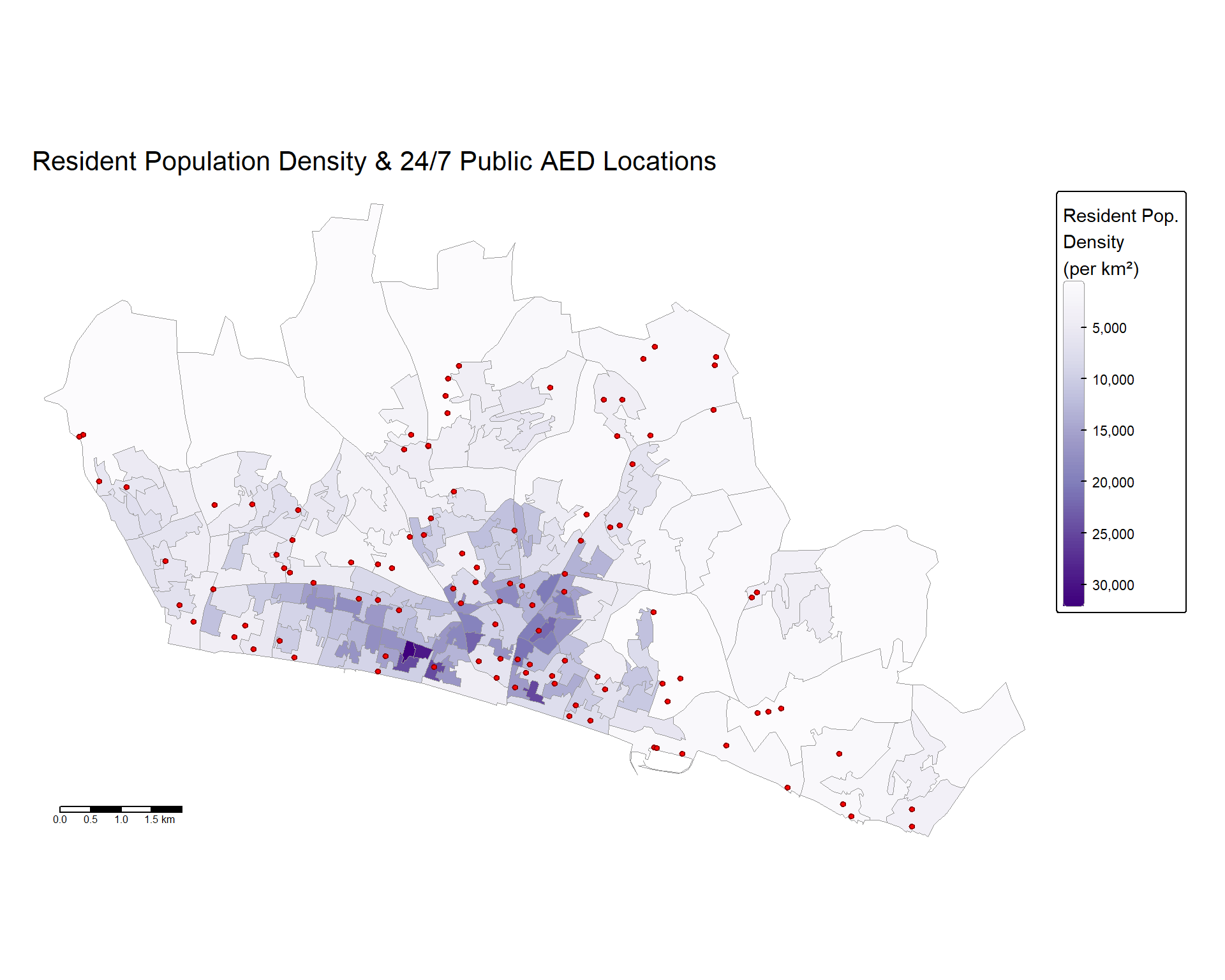
Zoom in to explore resident population density by LSOA. Click on LSOAs for population data, or on red markers for AED details.
# Create colour palette for resident density
pal_resident <- colorNumeric("Purples",
                              domain = bh_analysis$resident_density)

leaflet() %>%
  addProviderTiles(providers$CartoDB.Positron) %>%
  addPolygons(
    data = bh_analysis,
    fillColor = ~pal_resident(resident_density),
    fillOpacity = 0.6,
    color = "grey50",
    weight = 1,
    popup = ~paste0(
      "<strong>", LSOA21NM, "</strong><br>",
      "<em>Usual residents:</em> ",
      format(resident_pop, big.mark = ","), "<br>",
      "<em>Resident density:</em> ",
      format(round(resident_density), big.mark = ","), " per km²<br>",
      "<em>24/7 Public AEDs:</em> ", aed_count, "<br>",
      "<em>Resident priority rank:</em> ",
      resident_priority_rank, " of ", nrow(bh_analysis)
    ),
    group = "Resident Density"
  ) %>%
  addCircleMarkers(
    data = bh_247_sf,
    radius = 5,
    color = "darkred",
    fillColor = "red",
    fillOpacity = 0.8,
    weight = 1,
    popup = ~paste0(
      "<strong>", location_name, "</strong><br>",
      address_line1, "<br>",
      address_city, " ", address_post_code
    ),
    group = "24/7 Public AEDs"
  ) %>%
  addLegend(
    position = "bottomright",
    pal = pal_resident,
    values = bh_analysis$resident_density,
    title = "Resident Density<br>(per km²)"
  ) %>%
  addLayersControl(
    overlayGroups = c("Resident Density", "24/7 Public AEDs"),
    options = layersControlOptions(collapsed = FALSE)
)The resident priority score is calculated as: resident population density ÷ (number of existing 24/7 public AEDs + 1). LSOAs outlined in purple are the top 20 priority areas based on resident population demand.
bh_analysis <- bh_analysis %>%
  mutate(resident_top20 = resident_priority_rank <= 20)

# Colour palette for resident priority score
pal_res_priority <- colorNumeric("YlOrRd",
                                  domain = bh_analysis$resident_priority_score)

leaflet() %>%
  addProviderTiles(providers$CartoDB.Positron) %>%
  addPolygons(
    data = bh_analysis,
    fillColor = ~pal_res_priority(resident_priority_score),
    fillOpacity = 0.6,
    color = ~ifelse(resident_top20, "purple", "grey50"),
    weight = ~ifelse(resident_top20, 3, 1),
    popup = ~paste0(
      "<strong>", LSOA21NM, "</strong><br>",
      "<em>Resident priority rank:</em> <strong>",
      resident_priority_rank,
      "</strong> of ", nrow(bh_analysis), "<br>",
      "<em>Resident priority score:</em> ",
      format(round(resident_priority_score), big.mark = ","), "<br>",
      "<em>Resident density:</em> ",
      format(round(resident_density), big.mark = ","), " per km²<br>",
      "<em>Usual residents:</em> ",
      format(resident_pop, big.mark = ","), "<br>",
      "<em>24/7 Public AEDs:</em> ", aed_count
    ),
    group = "Resident Priority"
  ) %>%
  addCircleMarkers(
    data = bh_247_sf,
    radius = 4,
    color = "black",
    fillColor = "white",
    fillOpacity = 0.9,
    weight = 1.5,
    popup = ~paste0(
      "<strong>", location_name, "</strong><br>",
      address_line1, "<br>",
      address_city, " ", address_post_code
    ),
    group = "24/7 Public AEDs"
  ) %>%
  addLegend(
    position = "bottomright",
    pal = pal_res_priority,
    values = bh_analysis$resident_priority_score,
    title = "Resident Priority<br>Score"
  ) %>%
  addLayersControl(
    overlayGroups = c("Resident Priority", "24/7 Public AEDs"),
    options = layersControlOptions(collapsed = FALSE)
)The table below ranks all Brighton & Hove LSOAs by priority for new AED placement based on usual resident population density.
resident_priority_table <- bh_analysis %>%
  st_drop_geometry() %>%
  select(
    Rank = resident_priority_rank,
    LSOA = LSOA21NM,
    `Usual Residents` = resident_pop,
    `Resident Density (per km²)` = resident_density,
    `24/7 Public AEDs` = aed_count,
    `Priority Score` = resident_priority_score
  ) %>%
  arrange(Rank) %>%
  mutate(
    `Usual Residents` = format(`Usual Residents`, big.mark = ","),
    `Resident Density (per km²)` = format(round(`Resident Density (per km²)`),
                                            big.mark = ","),
    `Priority Score` = format(round(`Priority Score`), big.mark = ",")
  )

# Show top 20
resident_priority_table %>%
  head(20) %>%
  kable(align = c("r", "l", "r", "r", "r", "r")) %>%
  kable_styling(bootstrap_options = c("striped", "hover", "condensed"),
                full_width = FALSE) %>%
row_spec(0, bold = TRUE)| Rank | LSOA | Usual Residents | Resident Density (per km²) | 24/7 Public AEDs | Priority Score |
|---|---|---|---|---|---|
| 1 | Brighton and Hove 026B | 1,579 | 32,218 | 0 | 32,218 |
| 2 | Brighton and Hove 029C | 1,601 | 29,637 | 0 | 29,637 |
| 3 | Brighton and Hove 030B | 1,574 | 24,918 | 0 | 24,918 |
| 4 | Brighton and Hove 029B | 1,725 | 24,590 | 0 | 24,590 |
| 5 | Brighton and Hove 024E | 1,415 | 22,583 | 0 | 22,583 |
| 6 | Brighton and Hove 015D | 1,960 | 20,118 | 0 | 20,118 |
| 7 | Brighton and Hove 022C | 1,916 | 20,043 | 0 | 20,043 |
| 8 | Brighton and Hove 022E | 1,706 | 19,905 | 0 | 19,905 |
| 9 | Brighton and Hove 024D | 1,782 | 19,376 | 0 | 19,376 |
| 10 | Brighton and Hove 022A | 1,770 | 19,294 | 0 | 19,294 |
| 11 | Brighton and Hove 024B | 1,765 | 18,568 | 0 | 18,568 |
| 12 | Brighton and Hove 019C | 1,791 | 18,089 | 0 | 18,089 |
| 13 | Brighton and Hove 018B | 1,845 | 17,816 | 0 | 17,816 |
| 14 | Brighton and Hove 026E | 1,628 | 17,598 | 0 | 17,598 |
| 15 | Brighton and Hove 026C | 1,869 | 17,520 | 0 | 17,520 |
| 16 | Brighton and Hove 016C | 1,739 | 17,498 | 0 | 17,498 |
| 17 | Brighton and Hove 028B | 1,463 | 17,164 | 0 | 17,164 |
| 18 | Brighton and Hove 027F | 1,280 | 17,088 | 0 | 17,088 |
| 19 | Brighton and Hove 024C | 1,562 | 16,831 | 0 | 16,831 |
| 20 | Brighton and Hove 029E | 1,624 | 16,619 | 0 | 16,619 |
resident_priority_table %>%
  kable(align = c("r", "l", "r", "r", "r", "r")) %>%
  kable_styling(bootstrap_options = c("striped", "hover", "condensed"),
                full_width = FALSE) %>%
  row_spec(0, bold = TRUE) %>%
scroll_box(height = "400px")| Rank | LSOA | Usual Residents | Resident Density (per km²) | 24/7 Public AEDs | Priority Score |
|---|---|---|---|---|---|
| 1 | Brighton and Hove 026B | 1,579 | 32,218 | 0 | 32,218 |
| 2 | Brighton and Hove 029C | 1,601 | 29,637 | 0 | 29,637 |
| 3 | Brighton and Hove 030B | 1,574 | 24,918 | 0 | 24,918 |
| 4 | Brighton and Hove 029B | 1,725 | 24,590 | 0 | 24,590 |
| 5 | Brighton and Hove 024E | 1,415 | 22,583 | 0 | 22,583 |
| 6 | Brighton and Hove 015D | 1,960 | 20,118 | 0 | 20,118 |
| 7 | Brighton and Hove 022C | 1,916 | 20,043 | 0 | 20,043 |
| 8 | Brighton and Hove 022E | 1,706 | 19,905 | 0 | 19,905 |
| 9 | Brighton and Hove 024D | 1,782 | 19,376 | 0 | 19,376 |
| 10 | Brighton and Hove 022A | 1,770 | 19,294 | 0 | 19,294 |
| 11 | Brighton and Hove 024B | 1,765 | 18,568 | 0 | 18,568 |
| 12 | Brighton and Hove 019C | 1,791 | 18,089 | 0 | 18,089 |
| 13 | Brighton and Hove 018B | 1,845 | 17,816 | 0 | 17,816 |
| 14 | Brighton and Hove 026E | 1,628 | 17,598 | 0 | 17,598 |
| 15 | Brighton and Hove 026C | 1,869 | 17,520 | 0 | 17,520 |
| 16 | Brighton and Hove 016C | 1,739 | 17,498 | 0 | 17,498 |
| 17 | Brighton and Hove 028B | 1,463 | 17,164 | 0 | 17,164 |
| 18 | Brighton and Hove 027F | 1,280 | 17,088 | 0 | 17,088 |
| 19 | Brighton and Hove 024C | 1,562 | 16,831 | 0 | 16,831 |
| 20 | Brighton and Hove 029E | 1,624 | 16,619 | 0 | 16,619 |
| 21 | Brighton and Hove 019B | 1,767 | 16,362 | 0 | 16,362 |
| 22 | Brighton and Hove 016B | 1,689 | 15,905 | 0 | 15,905 |
| 23 | Brighton and Hove 022B | 1,880 | 15,603 | 0 | 15,603 |
| 24 | Brighton and Hove 010B | 1,866 | 13,507 | 0 | 13,507 |
| 25 | Brighton and Hove 018D | 1,745 | 13,281 | 0 | 13,281 |
| 26 | Brighton and Hove 027B | 1,545 | 13,232 | 0 | 13,232 |
| 27 | Brighton and Hove 016D | 1,898 | 13,048 | 0 | 13,048 |
| 28 | Brighton and Hove 026D | 1,576 | 12,830 | 0 | 12,830 |
| 29 | Brighton and Hove 020E | 1,804 | 12,686 | 0 | 12,686 |
| 30 | Brighton and Hove 029D | 1,674 | 24,783 | 1 | 12,392 |
| 31 | Brighton and Hove 020C | 1,540 | 12,110 | 0 | 12,110 |
| 32 | Brighton and Hove 010E | 1,583 | 11,978 | 0 | 11,978 |
| 33 | Brighton and Hove 025B | 1,514 | 11,605 | 0 | 11,605 |
| 34 | Brighton and Hove 019A | 1,684 | 11,604 | 0 | 11,604 |
| 35 | Brighton and Hove 018E | 1,499 | 11,586 | 0 | 11,586 |
| 36 | Brighton and Hove 021D | 1,723 | 11,556 | 0 | 11,556 |
| 37 | Brighton and Hove 010A | 1,704 | 11,278 | 0 | 11,278 |
| 38 | Brighton and Hove 031D | 1,469 | 11,089 | 0 | 11,089 |
| 39 | Brighton and Hove 022D | 1,684 | 21,886 | 1 | 10,943 |
| 40 | Brighton and Hove 025E | 1,609 | 10,847 | 0 | 10,847 |
| 41 | Brighton and Hove 032B | 1,928 | 10,805 | 0 | 10,805 |
| 42 | Brighton and Hove 030C | 2,126 | 21,007 | 1 | 10,503 |
| 43 | Brighton and Hove 023C | 1,555 | 10,485 | 0 | 10,485 |
| 44 | Brighton and Hove 028E | 1,514 | 10,432 | 0 | 10,432 |
| 45 | Brighton and Hove 028A | 1,580 | 10,010 | 0 | 10,010 |
| 46 | Brighton and Hove 020A | 1,608 | 9,882 | 0 | 9,882 |
| 47 | Brighton and Hove 029A | 1,614 | 9,829 | 0 | 9,829 |
| 48 | Brighton and Hove 014B | 1,405 | 9,798 | 0 | 9,798 |
| 49 | Brighton and Hove 014A | 1,593 | 9,774 | 0 | 9,774 |
| 50 | Brighton and Hove 010C | 1,323 | 9,610 | 0 | 9,610 |
| 51 | Brighton and Hove 013B | 1,387 | 9,569 | 0 | 9,569 |
| 52 | Brighton and Hove 027C | 2,423 | 9,430 | 0 | 9,430 |
| 53 | Brighton and Hove 015E | 1,755 | 18,322 | 1 | 9,161 |
| 54 | Brighton and Hove 023A | 1,723 | 9,027 | 0 | 9,027 |
| 55 | Brighton and Hove 020D | 1,792 | 8,334 | 0 | 8,334 |
| 56 | Brighton and Hove 019E | 1,850 | 8,315 | 0 | 8,315 |
| 57 | Brighton and Hove 030A | 1,950 | 15,999 | 1 | 8,000 |
| 58 | Brighton and Hove 025C | 1,500 | 7,760 | 0 | 7,760 |
| 59 | Brighton and Hove 026A | 1,528 | 15,502 | 1 | 7,751 |
| 60 | Brighton and Hove 031E | 1,615 | 7,499 | 0 | 7,499 |
| 61 | Brighton and Hove 014E | 2,140 | 14,966 | 1 | 7,483 |
| 62 | Brighton and Hove 011C | 1,696 | 7,478 | 0 | 7,478 |
| 63 | Brighton and Hove 015A | 1,905 | 14,913 | 1 | 7,457 |
| 64 | Brighton and Hove 008D | 1,710 | 7,183 | 0 | 7,183 |
| 65 | Brighton and Hove 012B | 1,315 | 7,078 | 0 | 7,078 |
| 66 | Brighton and Hove 031C | 1,893 | 14,060 | 1 | 7,030 |
| 67 | Brighton and Hove 012C | 1,524 | 6,875 | 0 | 6,875 |
| 68 | Brighton and Hove 015B | 1,730 | 13,412 | 1 | 6,706 |
| 69 | Brighton and Hove 008C | 1,884 | 6,569 | 0 | 6,569 |
| 70 | Brighton and Hove 012A | 1,659 | 6,564 | 0 | 6,564 |
| 71 | Brighton and Hove 006E | 1,588 | 6,300 | 0 | 6,300 |
| 72 | Brighton and Hove 030D | 1,788 | 12,450 | 1 | 6,225 |
| 73 | Brighton and Hove 004D | 1,619 | 6,173 | 0 | 6,173 |
| 74 | Brighton and Hove 012D | 1,587 | 6,153 | 0 | 6,153 |
| 75 | Brighton and Hove 015C | 1,617 | 12,117 | 1 | 6,058 |
| 76 | Brighton and Hove 009C | 1,544 | 6,044 | 0 | 6,044 |
| 77 | Brighton and Hove 011D | 1,707 | 12,073 | 1 | 6,036 |
| 78 | Brighton and Hove 005E | 1,557 | 5,925 | 0 | 5,925 |
| 79 | Brighton and Hove 004A | 1,554 | 5,898 | 0 | 5,898 |
| 80 | Brighton and Hove 032D | 1,931 | 5,887 | 0 | 5,887 |
| 81 | Brighton and Hove 024A | 1,942 | 17,489 | 2 | 5,830 |
| 82 | Brighton and Hove 010D | 1,595 | 11,577 | 1 | 5,789 |
| 83 | Brighton and Hove 007B | 1,319 | 5,692 | 0 | 5,692 |
| 84 | Brighton and Hove 006A | 1,540 | 5,678 | 0 | 5,678 |
| 85 | Brighton and Hove 020B | 1,906 | 11,209 | 1 | 5,604 |
| 86 | Brighton and Hove 008E | 1,734 | 5,550 | 0 | 5,550 |
| 87 | Brighton and Hove 007E | 1,581 | 5,330 | 0 | 5,330 |
| 88 | Brighton and Hove 001C | 1,586 | 5,091 | 0 | 5,091 |
| 89 | Brighton and Hove 031B | 1,547 | 9,992 | 1 | 4,996 |
| 90 | Brighton and Hove 023B | 1,489 | 9,953 | 1 | 4,976 |
| 91 | Brighton and Hove 005B | 1,419 | 4,926 | 0 | 4,926 |
| 92 | Brighton and Hove 018A | 1,677 | 4,770 | 0 | 4,770 |
| 93 | Brighton and Hove 001D | 1,548 | 4,756 | 0 | 4,756 |
| 94 | Brighton and Hove 027G | 1,860 | 9,480 | 1 | 4,740 |
| 95 | Brighton and Hove 011E | 1,639 | 9,444 | 1 | 4,722 |
| 96 | Brighton and Hove 025F | 1,632 | 4,595 | 0 | 4,595 |
| 97 | Brighton and Hove 028C | 1,388 | 8,994 | 1 | 4,497 |
| 98 | Brighton and Hove 018C | 1,937 | 13,434 | 2 | 4,478 |
| 99 | Brighton and Hove 008B | 1,588 | 4,458 | 0 | 4,458 |
| 100 | Brighton and Hove 017C | 1,508 | 4,345 | 0 | 4,345 |
| 101 | Brighton and Hove 013F | 1,604 | 4,335 | 0 | 4,335 |
| 102 | Brighton and Hove 013A | 1,538 | 4,197 | 0 | 4,197 |
| 103 | Brighton and Hove 004B | 1,916 | 4,033 | 0 | 4,033 |
| 104 | Brighton and Hove 017D | 1,782 | 4,021 | 0 | 4,021 |
| 105 | Brighton and Hove 005D | 1,319 | 3,975 | 0 | 3,975 |
| 106 | Brighton and Hove 027A | 1,783 | 3,923 | 0 | 3,923 |
| 107 | Brighton and Hove 001A | 1,444 | 3,824 | 0 | 3,824 |
| 108 | Brighton and Hove 025D | 1,344 | 3,719 | 0 | 3,719 |
| 109 | Brighton and Hove 009D | 1,391 | 3,689 | 0 | 3,689 |
| 110 | Brighton and Hove 013C | 1,552 | 3,626 | 0 | 3,626 |
| 111 | Brighton and Hove 019D | 1,799 | 10,827 | 2 | 3,609 |
| 112 | Brighton and Hove 006C | 1,689 | 7,213 | 1 | 3,607 |
| 113 | Brighton and Hove 021B | 1,634 | 6,911 | 1 | 3,455 |
| 114 | Brighton and Hove 033B | 1,811 | 3,319 | 0 | 3,319 |
| 115 | Brighton and Hove 011B | 1,692 | 3,202 | 0 | 3,202 |
| 116 | Brighton and Hove 021E | 1,668 | 6,317 | 1 | 3,159 |
| 117 | Brighton and Hove 002D | 1,477 | 6,099 | 1 | 3,049 |
| 118 | Brighton and Hove 028D | 1,631 | 5,937 | 1 | 2,969 |
| 119 | Brighton and Hove 007D | 1,517 | 2,938 | 0 | 2,938 |
| 120 | Brighton and Hove 012E | 1,695 | 5,773 | 1 | 2,886 |
| 121 | Brighton and Hove 023D | 1,719 | 5,367 | 1 | 2,684 |
| 122 | Brighton and Hove 007C | 1,494 | 2,672 | 0 | 2,672 |
| 123 | Brighton and Hove 014D | 1,810 | 7,845 | 2 | 2,615 |
| 124 | Brighton and Hove 031A | 1,555 | 7,340 | 2 | 2,447 |
| 125 | Brighton and Hove 013D | 1,471 | 4,411 | 1 | 2,206 |
| 126 | Brighton and Hove 009B | 1,770 | 6,521 | 2 | 2,174 |
| 127 | Brighton and Hove 032A | 1,743 | 6,501 | 2 | 2,167 |
| 128 | Brighton and Hove 003E | 1,812 | 4,219 | 1 | 2,110 |
| 129 | Brighton and Hove 013E | 1,529 | 5,682 | 2 | 1,894 |
| 130 | Brighton and Hove 021A | 1,853 | 3,719 | 1 | 1,860 |
| 131 | Brighton and Hove 005C | 1,419 | 5,416 | 2 | 1,805 |
| 132 | Brighton and Hove 030E | 1,733 | 7,964 | 4 | 1,593 |
| 133 | Brighton and Hove 027E | 1,846 | 6,323 | 3 | 1,581 |
| 134 | Brighton and Hove 033C | 1,466 | 1,570 | 0 | 1,570 |
| 135 | Brighton and Hove 016A | 1,837 | 4,643 | 2 | 1,548 |
| 136 | Brighton and Hove 009A | 1,651 | 1,531 | 0 | 1,531 |
| 137 | Brighton and Hove 003C | 1,514 | 2,785 | 1 | 1,392 |
| 138 | Brighton and Hove 009E | 1,491 | 1,376 | 0 | 1,376 |
| 139 | Brighton and Hove 003A | 1,592 | 3,552 | 2 | 1,184 |
| 140 | Brighton and Hove 001E | 1,627 | 1,151 | 0 | 1,151 |
| 141 | Brighton and Hove 006B | 1,515 | 2,276 | 1 | 1,138 |
| 142 | Brighton and Hove 014C | 1,607 | 3,398 | 2 | 1,133 |
| 143 | Brighton and Hove 004C | 1,551 | 2,261 | 1 | 1,130 |
| 144 | Brighton and Hove 033E | 1,973 | 3,383 | 2 | 1,128 |
| 145 | Brighton and Hove 017A | 1,595 | 3,247 | 2 | 1,082 |
| 146 | Brighton and Hove 001B | 1,585 | 2,111 | 1 | 1,055 |
| 147 | Brighton and Hove 002A | 2,330 | 4,101 | 3 | 1,025 |
| 148 | Brighton and Hove 021C | 1,766 | 3,907 | 3 | 977 |
| 149 | Brighton and Hove 017F | 1,790 | 937 | 0 | 937 |
| 150 | Brighton and Hove 033A | 1,545 | 894 | 0 | 894 |
| 151 | Brighton and Hove 017B | 1,724 | 843 | 0 | 843 |
| 152 | Brighton and Hove 007A | 1,673 | 2,143 | 2 | 714 |
| 153 | Brighton and Hove 002C | 2,142 | 1,110 | 1 | 555 |
| 154 | Brighton and Hove 011A | 1,651 | 2,132 | 3 | 533 |
| 155 | Brighton and Hove 017E | 1,375 | 431 | 0 | 431 |
| 156 | Brighton and Hove 008A | 1,631 | 681 | 1 | 340 |
| 157 | Brighton and Hove 006D | 1,419 | 331 | 0 | 331 |
| 158 | Brighton and Hove 033D | 1,716 | 1,195 | 3 | 299 |
| 159 | Brighton and Hove 003D | 1,491 | 291 | 0 | 291 |
| 160 | Brighton and Hove 002B | 4,165 | 1,266 | 5 | 211 |
| 161 | Brighton and Hove 032C | 2,204 | 1,190 | 5 | 198 |
| 162 | Brighton and Hove 033F | 1,647 | 578 | 3 | 144 |
| 163 | Brighton and Hove 025A | 1,491 | 608 | 4 | 122 |
| 164 | Brighton and Hove 005A | 1,439 | 318 | 2 | 106 |
| 165 | Brighton and Hove 003B | 1,653 | 445 | 4 | 89 |
This map shows all LSOAs coloured by resident population priority rank (darker purple = higher priority), with existing 24/7 public AED locations (red markers) and OpenStreetMap telephone box locations (green markers).
# Colour palette: rank 1 = darkest, highest rank = lightest
pal_res_rank <- colorNumeric(
  palette = "Purples",
  domain = bh_analysis$resident_priority_rank,
  reverse = TRUE
)

leaflet() %>%
  addProviderTiles(providers$CartoDB.Positron) %>%
  addPolygons(
    data = bh_analysis,
    fillColor = ~pal_res_rank(resident_priority_rank),
    fillOpacity = 0.5,
    color = "grey50",
    weight = 1,
    popup = ~paste0(
      "<strong>", LSOA21NM, "</strong><br>",
      "<em>Resident priority rank:</em> <strong>",
      resident_priority_rank,
      "</strong> of ", nrow(bh_analysis), "<br>",
      "<em>Resident priority score:</em> ",
      format(round(resident_priority_score), big.mark = ","), "<br>",
      "<em>Resident density:</em> ",
      format(round(resident_density), big.mark = ","), " per km²<br>",
      "<em>Usual residents:</em> ",
      format(resident_pop, big.mark = ","), "<br>",
      "<em>24/7 Public AEDs:</em> ", aed_count
    ),
    group = "Resident Priority Ranking"
  ) %>%
  addCircleMarkers(
    data = bh_247_sf,
    radius = 5,
    color = "darkred",
    fillColor = "red",
    fillOpacity = 0.8,
    weight = 1,
    popup = ~paste0(
      "<strong>", location_name, "</strong><br>",
      address_line1, "<br>",
      address_city, " ", address_post_code
    ),
    group = "24/7 Public AEDs"
  ) %>%
  addCircleMarkers(
    data = phone_sf,
    radius = 5,
    color = "darkgreen",
    fillColor = "#2ca02c",
    fillOpacity = 0.8,
    weight = 1,
    popup = ~paste0(
      "<strong>Telephone Box</strong><br>",
      "<em>OSM ID:</em> ", id
    ),
    group = "Telephone Boxes (OSM)"
  ) %>%
  addLegend(
    position = "bottomright",
    pal = pal_res_rank,
    values = bh_analysis$resident_priority_rank,
    title = "Resident<br>Priority Rank",
    labFormat = labelFormat(transform = function(x) round(x))
  ) %>%
  addLegend(
    position = "bottomright",
    colors = c("red", "#2ca02c"),
    labels = c("24/7 Public AED", "Telephone Box"),
    title = "Points"
  ) %>%
  addLayersControl(
    overlayGroups = c("Resident Priority Ranking", "24/7 Public AEDs",
                      "Telephone Boxes (OSM)"),
    options = layersControlOptions(collapsed = FALSE)
)Different population measures can lead to different conclusions about where AEDs are most needed. The workday population reflects daytime demand (offices, shops, transport hubs), while the resident population reflects overnight, evening, and weekend demand (homes, residential streets). Comparing the two reveals which areas are consistently high-priority and which shift depending on the measure used.
comparison_df <- bh_analysis %>%
  st_drop_geometry() %>%
  select(LSOA21NM, workday_density, resident_density, aed_count,
         priority_rank, resident_priority_rank)

ggplot(comparison_df,
       aes(x = workday_density, y = resident_density)) +
  geom_point(aes(colour = factor(pmin(aed_count, 3))),
             size = 2.5, alpha = 0.7) +
  geom_abline(intercept = 0, slope = 1,
              linetype = "dashed", colour = "grey40") +
  scale_colour_manual(
    values = c("0" = "#d73027", "1" = "#fee08b",
               "2" = "#91cf60", "3" = "#1a9850"),
    labels = c("0" = "0", "1" = "1", "2" = "2", "3" = "3+"),
    name = "24/7 Public\nAEDs"
  ) +
  scale_x_continuous(labels = scales::comma) +
  scale_y_continuous(labels = scales::comma) +
  labs(
    title = "Workday vs. Resident Population Density by LSOA",
    subtitle = "Points above the diagonal have higher resident than workday density",
    x = "Workday Population Density (per km²)",
    y = "Resident Population Density (per km²)"
  ) +
  theme_minimal() +
  theme(legend.position = "right")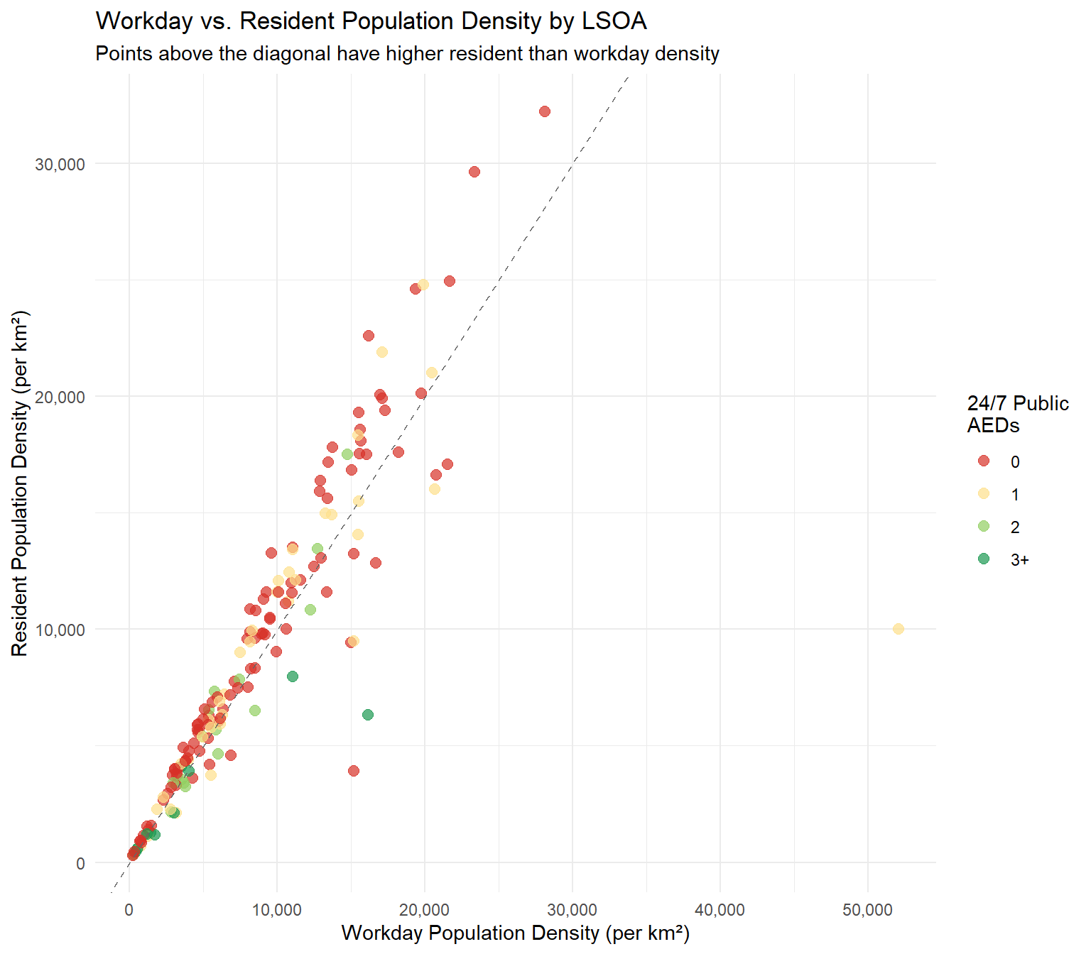
LSOAs above the dashed line have higher resident density than workday density — predominantly residential areas. LSOAs below the line attract more people during the day than they house — commercial, retail, or transport hubs. Red points (no AEDs) in either high-density zone indicate gaps in coverage.
The table below shows LSOAs where the priority ranking changes most between the two measures. A large positive rank difference means the LSOA is ranked as much higher priority by the resident analysis than the workday analysis (i.e. it is a densely populated residential area that is less busy during the day). A large negative difference means the reverse — a daytime hotspot that is less densely populated residentially.
rank_changes <- bh_analysis %>%
  st_drop_geometry() %>%
  mutate(
    rank_diff = priority_rank - resident_priority_rank
  ) %>%
  select(
    LSOA = LSOA21NM,
    `Workday Rank` = priority_rank,
    `Resident Rank` = resident_priority_rank,
    `Rank Difference` = rank_diff,
    `Workday Density` = workday_density,
    `Resident Density` = resident_density,
    `24/7 Public AEDs` = aed_count
  ) %>%
  arrange(desc(abs(`Rank Difference`)))

# Show top 20 largest rank changes
rank_changes %>%
  head(20) %>%
  mutate(
    `Workday Density` = format(round(`Workday Density`), big.mark = ","),
    `Resident Density` = format(round(`Resident Density`), big.mark = ",")
  ) %>%
  kable(align = c("l", "r", "r", "r", "r", "r", "r")) %>%
  kable_styling(bootstrap_options = c("striped", "hover", "condensed"),
                full_width = FALSE) %>%
row_spec(0, bold = TRUE)| LSOA | Workday Rank | Resident Rank | Rank Difference | Workday Density | Resident Density | 24/7 Public AEDs |
|---|---|---|---|---|---|---|
| Brighton and Hove 031B | 2 | 89 | -87 | 52,028 | 9,992 | 1 |
| Brighton and Hove 027A | 20 | 106 | -86 | 15,200 | 3,923 | 0 |
| Brighton and Hove 027E | 101 | 133 | -32 | 16,133 | 6,323 | 3 |
| Brighton and Hove 027G | 63 | 94 | -31 | 15,204 | 9,480 | 1 |
| Brighton and Hove 025F | 66 | 96 | -30 | 6,862 | 4,595 | 0 |
| Brighton and Hove 027C | 23 | 52 | -29 | 14,996 | 9,430 | 0 |
| Brighton and Hove 013A | 77 | 102 | -25 | 5,453 | 4,197 | 0 |
| Brighton and Hove 030A | 38 | 57 | -19 | 20,648 | 15,999 | 1 |
| Brighton and Hove 018D | 43 | 25 | 18 | 9,598 | 13,281 | 0 |
| Brighton and Hove 025E | 57 | 40 | 17 | 8,174 | 10,847 | 0 |
| Brighton and Hove 026D | 13 | 28 | -15 | 16,704 | 12,830 | 0 |
| Brighton and Hove 013C | 95 | 110 | -15 | 4,295 | 3,626 | 0 |
| Brighton and Hove 005B | 106 | 91 | 15 | 3,679 | 4,926 | 0 |
| Brighton and Hove 029E | 6 | 20 | -14 | 20,784 | 16,619 | 0 |
| Brighton and Hove 025B | 46 | 33 | 13 | 9,292 | 11,605 | 0 |
| Brighton and Hove 019D | 98 | 111 | -13 | 12,244 | 10,827 | 2 |
| Brighton and Hove 022D | 52 | 39 | 13 | 17,117 | 21,886 | 1 |
| Brighton and Hove 012A | 83 | 70 | 13 | 5,107 | 6,564 | 0 |
| Brighton and Hove 004A | 92 | 79 | 13 | 4,623 | 5,898 | 0 |
| Brighton and Hove 023A | 41 | 54 | -13 | 9,958 | 9,027 | 0 |
This map visualises how priority rankings shift between the two population measures. Blue LSOAs are ranked as higher priority under the workday analysis (daytime hotspots); red LSOAs are ranked as higher priority under the resident analysis (residential demand). Neutral colours indicate consistent priority under both measures.
bh_analysis <- bh_analysis %>%
  mutate(rank_diff = priority_rank - resident_priority_rank)

# Diverging palette: blue = workday priority higher, red = resident priority higher
max_abs_diff <- max(abs(bh_analysis$rank_diff), na.rm = TRUE)
pal_diff <- colorNumeric(
  palette = "RdBu",
  domain = c(-max_abs_diff, max_abs_diff),
  reverse = TRUE
)

leaflet() %>%
  addProviderTiles(providers$CartoDB.Positron) %>%
  addPolygons(
    data = bh_analysis,
    fillColor = ~pal_diff(rank_diff),
    fillOpacity = 0.6,
    color = "grey50",
    weight = 1,
    popup = ~paste0(
      "<strong>", LSOA21NM, "</strong><br>",
      "<em>Workday priority rank:</em> ", priority_rank, "<br>",
      "<em>Resident priority rank:</em> ", resident_priority_rank, "<br>",
      "<em>Rank difference:</em> <strong>",
      ifelse(rank_diff > 0, paste0("+", rank_diff), rank_diff),
      "</strong><br>",
      "<hr style='margin:4px 0'>",
      "<em>Workday density:</em> ",
      format(round(workday_density), big.mark = ","), " per km²<br>",
      "<em>Resident density:</em> ",
      format(round(resident_density), big.mark = ","), " per km²<br>",
      "<em>24/7 Public AEDs:</em> ", aed_count
    ),
    group = "Rank Difference"
  ) %>%
  addCircleMarkers(
    data = bh_247_sf,
    radius = 4,
    color = "black",
    fillColor = "white",
    fillOpacity = 0.9,
    weight = 1.5,
    popup = ~paste0(
      "<strong>", location_name, "</strong><br>",
      address_line1, "<br>",
      address_city, " ", address_post_code
    ),
    group = "24/7 Public AEDs"
  ) %>%
  addLegend(
    position = "bottomright",
    pal = pal_diff,
    values = bh_analysis$rank_diff,
    title = "Rank Difference<br>(Workday − Resident)",
    labFormat = labelFormat(
      transform = function(x) round(x)
    )
  ) %>%
  addLayersControl(
    overlayGroups = c("Rank Difference", "24/7 Public AEDs"),
    options = layersControlOptions(collapsed = FALSE)
)This map combines both population measures into a single priority ranking by averaging the workday and resident priority ranks. This gives equal weight to daytime and residential demand, producing a balanced view of where new AEDs are most needed across all times of day. Darker shading indicates higher combined priority. LSOAs outlined in red are the top 20 under the combined ranking.
# Compute combined priority: average of the two ranks (lower = higher priority)
bh_analysis <- bh_analysis %>%
  mutate(
    combined_avg_rank = (priority_rank + resident_priority_rank) / 2,
    combined_priority_rank = rank(combined_avg_rank, ties.method = "first"),
    combined_top20 = combined_priority_rank <= 20
  )

# Colour palette: rank 1 = darkest
pal_combined <- colorNumeric(
  palette = "YlOrRd",
  domain = bh_analysis$combined_priority_rank,
  reverse = TRUE
)

leaflet() %>%
  addProviderTiles(providers$CartoDB.Positron) %>%
  addPolygons(
    data = bh_analysis,
    fillColor = ~pal_combined(combined_priority_rank),
    fillOpacity = 0.5,
    color = ~ifelse(combined_top20, "red", "grey50"),
    weight = ~ifelse(combined_top20, 3, 1),
    popup = ~paste0(
      "<strong>", LSOA21NM, "</strong><br>",
      "<em>Combined priority rank:</em> <strong>",
      combined_priority_rank,
      "</strong> of ", nrow(bh_analysis), "<br>",
      "<em>Workday rank:</em> ", priority_rank,
      " | <em>Resident rank:</em> ", resident_priority_rank, "<br>",
      "<hr style='margin:4px 0'>",
      "<em>Workday density:</em> ",
      format(round(workday_density), big.mark = ","), " per km²<br>",
      "<em>Resident density:</em> ",
      format(round(resident_density), big.mark = ","), " per km²<br>",
      "<em>24/7 Public AEDs:</em> ", aed_count
    ),
    group = "Combined Priority"
  ) %>%
  addCircleMarkers(
    data = bh_247_sf,
    radius = 5,
    color = "darkred",
    fillColor = "red",
    fillOpacity = 0.8,
    weight = 1,
    popup = ~paste0(
      "<strong>", location_name, "</strong><br>",
      address_line1, "<br>",
      address_city, " ", address_post_code
    ),
    group = "24/7 Public AEDs"
  ) %>%
  addCircleMarkers(
    data = phone_sf,
    radius = 5,
    color = "darkgreen",
    fillColor = "#2ca02c",
    fillOpacity = 0.8,
    weight = 1,
    popup = ~paste0(
      "<strong>Telephone Box</strong><br>",
      "<em>OSM ID:</em> ", id
    ),
    group = "Telephone Boxes (OSM)"
  ) %>%
  addLegend(
    position = "bottomright",
    pal = pal_combined,
    values = bh_analysis$combined_priority_rank,
    title = "Combined<br>Priority Rank",
    labFormat = labelFormat(transform = function(x) round(x))
  ) %>%
  addLegend(
    position = "bottomright",
    colors = c("red", "#2ca02c"),
    labels = c("24/7 Public AED", "Telephone Box"),
    title = "Points"
  ) %>%
  addLayersControl(
    overlayGroups = c("Combined Priority", "24/7 Public AEDs",
                      "Telephone Boxes (OSM)"),
    options = layersControlOptions(collapsed = FALSE)
)combined_table <- bh_analysis %>%
st_drop_geometry() %>%
select(
`Combined Rank` = combined_priority_rank,
LSOA = LSOA21NM,
`Workday Rank` = priority_rank,
`Resident Rank` = resident_priority_rank,
`Workday Density` = workday_density,
`Resident Density` = resident_density,
`24/7 Public AEDs` = aed_count
) %>%
arrange(`Combined Rank`) %>%
mutate(
`Workday Density` = format(round(`Workday Density`), big.mark = ","),
`Resident Density` = format(round(`Resident Density`), big.mark = ",")
)
combined_table %>%
head(20) %>%
kable(align = c("r", "l", "r", "r", "r", "r", "r")) %>%
kable_styling(bootstrap_options = c("striped", "hover", "condensed"),
full_width = FALSE) %>%
row_spec(0, bold = TRUE)| Combined Rank | LSOA | Workday Rank | Resident Rank | Workday Density | Resident Density | 24/7 Public AEDs |
|---|---|---|---|---|---|---|
| 1 | Brighton and Hove 026B | 1 | 1 | 28,107 | 32,218 | 0 |
| 2 | Brighton and Hove 029C | 3 | 2 | 23,370 | 29,637 | 0 |
| 3 | Brighton and Hove 030B | 4 | 3 | 21,688 | 24,918 | 0 |
| 4 | Brighton and Hove 029B | 8 | 4 | 19,366 | 24,590 | 0 |
| 5 | Brighton and Hove 015D | 7 | 6 | 19,733 | 20,118 | 0 |
| 6 | Brighton and Hove 022C | 12 | 7 | 16,954 | 20,043 | 0 |
| 7 | Brighton and Hove 022E | 11 | 8 | 17,129 | 19,905 | 0 |
| 8 | Brighton and Hove 024D | 10 | 9 | 17,287 | 19,376 | 0 |
| 9 | Brighton and Hove 024E | 14 | 5 | 16,196 | 22,583 | 0 |
| 10 | Brighton and Hove 026E | 9 | 14 | 18,232 | 17,598 | 0 |
| 11 | Brighton and Hove 027F | 5 | 18 | 21,522 | 17,088 | 0 |
| 12 | Brighton and Hove 029E | 6 | 20 | 20,784 | 16,619 | 0 |
| 13 | Brighton and Hove 019C | 16 | 12 | 15,691 | 18,089 | 0 |
| 14 | Brighton and Hove 024B | 17 | 11 | 15,646 | 18,568 | 0 |
| 15 | Brighton and Hove 022A | 19 | 10 | 15,520 | 19,294 | 0 |
| 16 | Brighton and Hove 016C | 15 | 16 | 16,043 | 17,498 | 0 |
| 17 | Brighton and Hove 026C | 18 | 15 | 15,557 | 17,520 | 0 |
| 18 | Brighton and Hove 018B | 24 | 13 | 13,752 | 17,816 | 0 |
| 19 | Brighton and Hove 026D | 13 | 28 | 16,704 | 12,830 | 0 |
| 20 | Brighton and Hove 024C | 22 | 19 | 15,032 | 16,831 | 0 |
LSOAs that rank in the top 20 under both workday and resident population analyses represent the most robust candidates for new AED placement — they have high demand regardless of which population measure is used.
consistent_top <- bh_analysis %>%
  st_drop_geometry() %>%
  filter(priority_rank <= 20, resident_priority_rank <= 20) %>%
  select(
    LSOA = LSOA21NM,
    `Workday Rank` = priority_rank,
    `Resident Rank` = resident_priority_rank,
    `Workday Density` = workday_density,
    `Resident Density` = resident_density,
    `24/7 Public AEDs` = aed_count
  ) %>%
  arrange(`Workday Rank`) %>%
  mutate(
    `Workday Density` = format(round(`Workday Density`), big.mark = ","),
    `Resident Density` = format(round(`Resident Density`), big.mark = ",")
  )

n_consistent <- nrow(consistent_top)

cat(n_consistent, "LSOAs appear in the top 20 under both measures:\n\n")
17 LSOAs appear in the top 20 under both measures:consistent_top %>%
kable(align = c("l", "r", "r", "r", "r", "r")) %>%
kable_styling(bootstrap_options = c("striped", "hover", "condensed"),
full_width = FALSE) %>%
row_spec(0, bold = TRUE)| LSOA | Workday Rank | Resident Rank | Workday Density | Resident Density | 24/7 Public AEDs |
|---|---|---|---|---|---|
| Brighton and Hove 026B | 1 | 1 | 28,107 | 32,218 | 0 |
| Brighton and Hove 029C | 3 | 2 | 23,370 | 29,637 | 0 |
| Brighton and Hove 030B | 4 | 3 | 21,688 | 24,918 | 0 |
| Brighton and Hove 027F | 5 | 18 | 21,522 | 17,088 | 0 |
| Brighton and Hove 029E | 6 | 20 | 20,784 | 16,619 | 0 |
| Brighton and Hove 015D | 7 | 6 | 19,733 | 20,118 | 0 |
| Brighton and Hove 029B | 8 | 4 | 19,366 | 24,590 | 0 |
| Brighton and Hove 026E | 9 | 14 | 18,232 | 17,598 | 0 |
| Brighton and Hove 024D | 10 | 9 | 17,287 | 19,376 | 0 |
| Brighton and Hove 022E | 11 | 8 | 17,129 | 19,905 | 0 |
| Brighton and Hove 022C | 12 | 7 | 16,954 | 20,043 | 0 |
| Brighton and Hove 024E | 14 | 5 | 16,196 | 22,583 | 0 |
| Brighton and Hove 016C | 15 | 16 | 16,043 | 17,498 | 0 |
| Brighton and Hove 019C | 16 | 12 | 15,691 | 18,089 | 0 |
| Brighton and Hove 024B | 17 | 11 | 15,646 | 18,568 | 0 |
| Brighton and Hove 026C | 18 | 15 | 15,557 | 17,520 | 0 |
| Brighton and Hove 022A | 19 | 10 | 15,520 | 19,294 | 0 |
The map below highlights the top 15 LSOAs from the combined priority ranking that also appear in the top 20 under both the workday and resident analyses. These are grouped into three tiers to help identify the most urgent candidates for new AED provision.
library(leaflet)
library(dplyr)

# 1. DATA PREPARATION
# Ensure top15 is created correctly in the current session
bh_analysis <- bh_analysis %>%
  mutate(consistent = priority_rank <= 20 & resident_priority_rank <= 20)

top15 <- bh_analysis %>%
  filter(consistent) %>%
  arrange(combined_priority_rank) %>%
  head(15) %>%
  mutate(
    tier = case_when(
      row_number() <= 5  ~ "Top 5",
      row_number() <= 10 ~ "6th–10th",
      TRUE               ~ "11th–15th"
    ),
    tier = factor(tier, levels = c("Top 5", "6th–10th", "11th–15th"))
  )

bg_lsoas <- bh_analysis %>% filter(!LSOA21CD %in% top15$LSOA21CD)

# 2. COLOR PALETTE
# Using ColorBrewer-style "YlOrRd" logic for a clear heat fade
pal <- colorFactor(
  palette = c("#d7191c", "#fdae61", "#ffffbf"),
  levels = c("Top 5", "6th–10th", "11th–15th")
)

# 3. MAP GENERATION
leaflet() %>%
  addProviderTiles(providers$CartoDB.Positron) %>%

  # Background: All other LSOAs
  addPolygons(
    data = bg_lsoas,
    fillColor = "#e0e0e0",
    fillOpacity = 0.3,
    color = "grey70",
    weight = 0.5,
    popup = ~paste0("<strong>", LSOA21NM, "</strong>"),
    group = "Other LSOAs"
  ) %>%

  # Foreground: Top 15 Priority LSOAs
  addPolygons(
    data = top15,
    fillColor = ~pal(tier),
    fillOpacity = 0.7,
    color = "black",
    weight = 2,
    popup = ~paste0(
      "<strong>", LSOA21NM, "</strong><br>",
      "<em>Tier:</em> <strong>", tier, "</strong><br>",
      "<em>Combined rank:</em> ", combined_priority_rank, "<br>",
      "<em>Workday rank:</em> ", priority_rank,
      " | <em>Resident rank:</em> ", resident_priority_rank, "<br>",
      "<hr style='margin:4px 0'>",
      "<em>Workday density:</em> ", format(round(workday_density), big.mark = ","), " per km²<br>",
      "<em>Resident density:</em> ", format(round(resident_density), big.mark = ","), " per km²<br>",
      "<em>24/7 Public AEDs:</em> ", aed_count
    ),
    group = "Top 15 Priority LSOAs"
  ) %>%

  # Points: 24/7 Public AEDs
  addCircleMarkers(
    data = bh_247_sf,
    radius = 4,
    color = "black",
    fillColor = "white",
    fillOpacity = 0.9,
    weight = 1.5,
    group = "24/7 Public AEDs"
  ) %>%

  # Points: Telephone Boxes
  addCircleMarkers(
    data = phone_sf,
    radius = 5,
    color = "darkgreen",
    fillColor = "#2ca02c",
    fillOpacity = 0.8,
    weight = 1,
    popup = ~paste0("<strong>Telephone Box</strong>"),
    group = "Telephone Boxes (OSM)" # This name must match the one below
  ) %>%

  # Legend
  addLegend(
    position = "bottomright",
    pal = pal,
    values = top15$tier,
    title = "Priority Tier",
    opacity = 0.7
  ) %>%

  # UPDATED: Added "Telephone Boxes (OSM)" to the overlayGroups
  addLayersControl(
    overlayGroups = c(
      "Top 15 Priority LSOAs",
      "Other LSOAs",
      "24/7 Public AEDs",
      "Telephone Boxes (OSM)"
    ),
    options = layersControlOptions(collapsed = FALSE)
)Key findings:
Data sourced from The Circuit, ONS Census 2021 Workday Population, and ONS Census 2021 Usual Resident Population. Is this an emergency? This website is used to locate defibrillators, but it is not intended for use in an emergency. If you require urgent medical assistance, call 999 now.