Foundations of Geospatial Analysis
November 21, 2023
About Me
![]()
Professor of Urban Analytics @ Bartlett Centre for Advanced Spatial Analysis (CASA), UCL
Geographer by background - ex-Secondary School Teacher - back in HE for 16+ years
Taught GIS / Spatial Data Science at postgrad level for last 11 years
Where? (absolute)
Everything happens somewhere
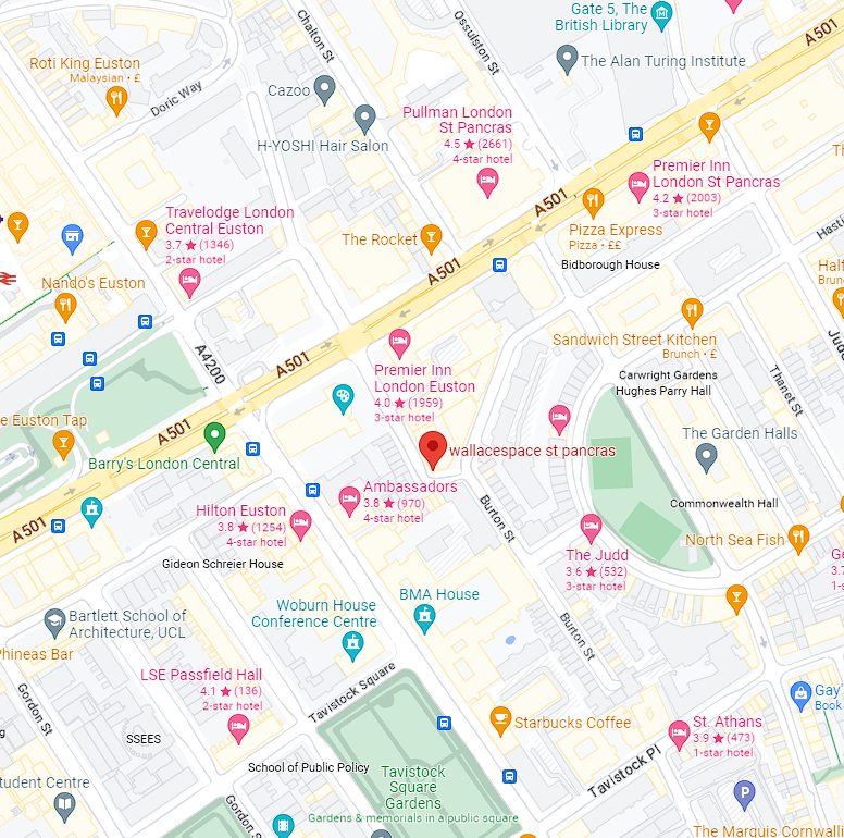
- We’re here: Wallspace, 22 Duke’s Road, Camden, London, England, *Europe, Northern Hemisphere, Earth
Where? (absolute)
- How do we know exactly where?
Where? Coordinate Reference Systems
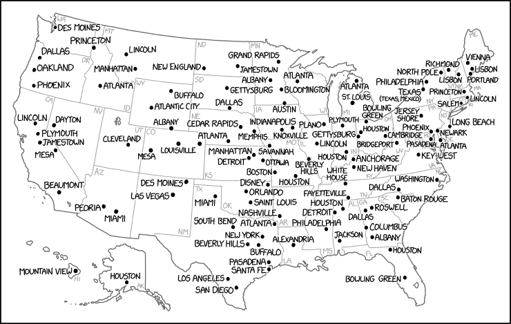
More reliable than names (that are rarely unique or reference fuzzy locations), are coordinates
The earth is roughly spherical and points anywhere on its surface can be described using the World Geodetic System (WGS) - a geographic (spherical) coordinate system
Points can be referenced according to their position on a grid of latitudes (degrees north or south of the equator) and longitudes (degrees east or west of the Prime - Greenwich - meridian)
The last major revision of the World Geodetic System was in 1984 and WGS84 is still used today as the standard system for references places on the globe.
Where? Coordinate Reference Systems
Projected Coordinate Reference Systems convert the 3D globe to a 2D plane and can do so in a huge variety of different ways
Most national mapping agencies have their own projected coordinate systems - in Britain the Ordnance Survey maintain the British National Grid which locates places according to 6-digit Easting and Northing coordinates
Every coordinate system can be referenced by its EPSG code, e.g. WGS84 = 4326 or British National Grid = 27700 with mathematical transformations to convert between them
![]()
Where? Describing and Locating Things with Coordinates
Once we have a coordinate reference system we can locate objects accurately in space
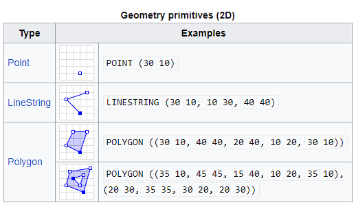
Most objects that spatial data scientists are concerned with (apart from gridded representations, which we will ignore for now!) can be simplified to either a point, a line or a polygon in that space
Polygons and lines are just multiple point coordinates joined together!
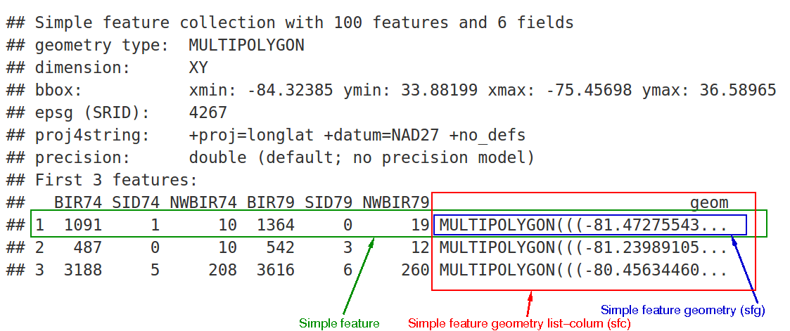
The examples on the right store geometries in the ‘well-known-text’ (WKT) format for representing vector (point, line, polygon) geometries
Storing where - managing spatial data
Impossible to talk about spatial data without mentioning the shapefile
Developed in the 1980s by ESRI and has become, pretty much, the de facto standard for storing and sharing spatial data - even though it’s a terrible format!
Shapefiles store geometries (shapes) and attributes (information about those shapes)
Not a single file, actually a collection of files
.shp - geometries
.shx - index
.dbf - attributes
+some others!
Superseded by LOTS of alternative formats - geojson (web), GeoPackage (everything) which do the same thing in better ways for different applications

Storing where - Simple Features
Simple Features - OGC (Open Geospatial Consortium) standard that specifies a common storage and access model for 2D geometries
2 part standard:
Part 1 - Common Architecture defining geometries, attributes etc. via WKT
Part 2 - supports storage, retrieval, query and update of simple geospatial feature collections via SQL (structured query language – been around since the 1970s)
Simple Features implemented in most spatially enabled database management systems (e.g. PostGIS extension for PostgreSQL, Oracle Spatial etc.)
sfpackage in R enables storage of spatial data and attributes in a single data frame object
Where? Relative - Tobler’s First Law of Geography
“Everything is related to everything else, but near things are more related than distant things.”

This observation underpins much of what spatial data scientists do
Being able to locate something in space, relative to something else, allows us to:
explain why something may be occurring where it is
make better predictions about nearby or further away things
Underpins the whole Geodeomographics (customer segmentation) industry!!

Where? Relative - John Snow’s Cholera Map

Where? Relative - Defining ‘near’ and ‘distant’
Near and distant can mean different things in different contexts
- the furthest one would travel to buy a pint of milk is somewhat different to furthest one might be willing to commute for a job
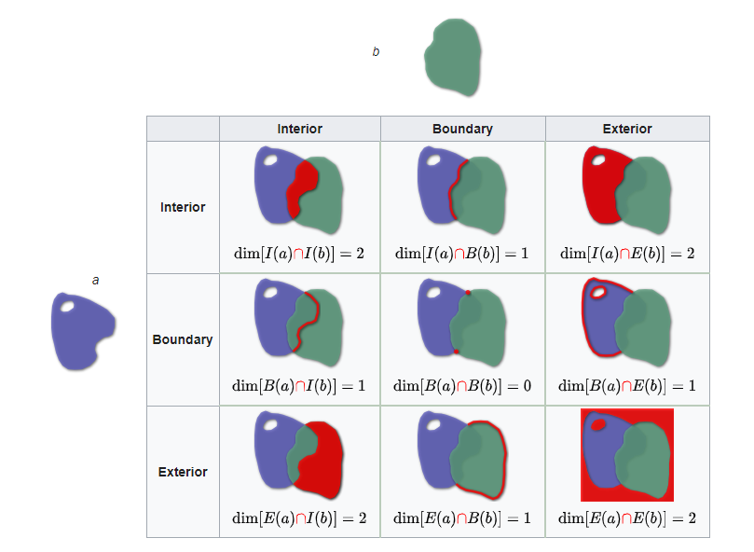
In spatial data science one way of separating near from distant can simply be to define their topological relationship - Dimensionally Extended 9-Intersection Model (DE-9IM) is the standard topological model used in GIS
Touching or overlapping objects = ‘near’
Where? Relative - Exploring Near and Distant
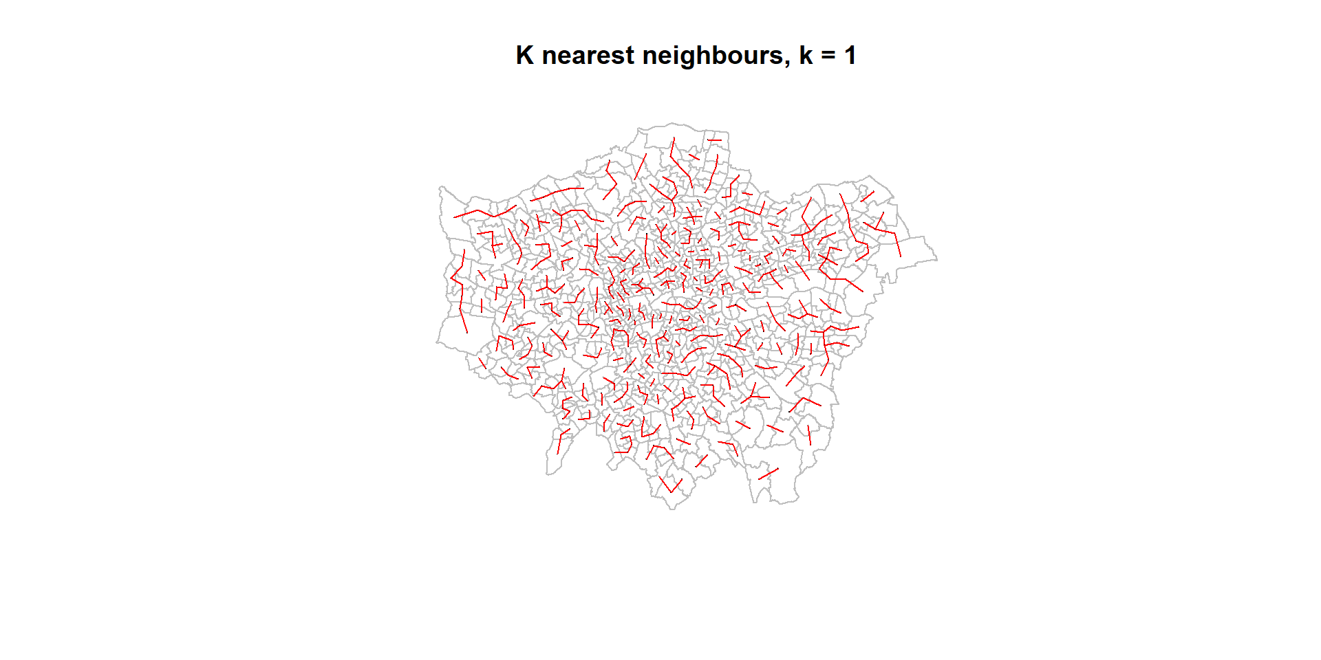
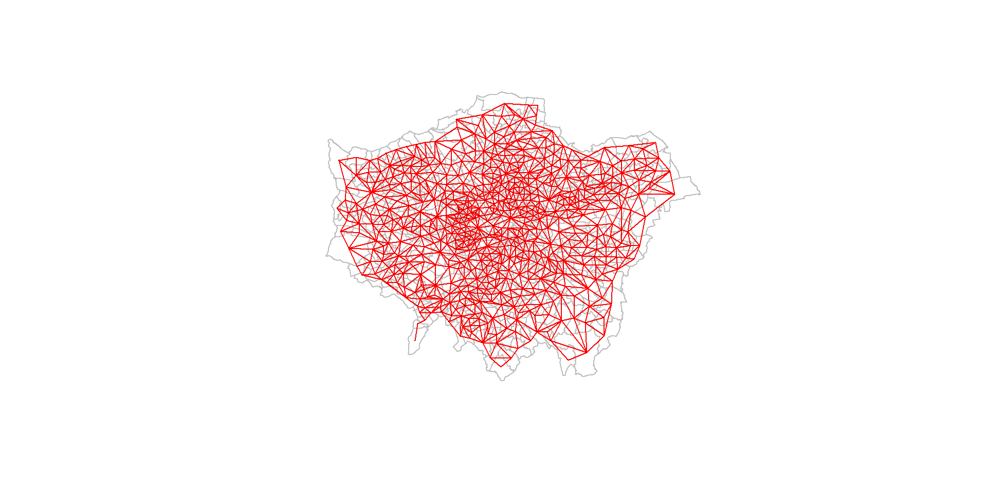
If we measure the distance from the centre (centroid) of one ward to another, then we might decide that the 1st, 2nd, 3rd, kth. closest wards are near, the others are far
These neighbour relationships can be stored in an \(n*n\) ‘spatial weights’ matrix
The
spdeppackage in R will calculate a range of spatial weights matrices given a set of geometries
Where? Relative - Exploring Near and Distant
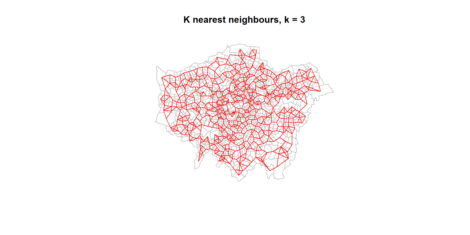
- We can then decide to include the “k” nearest neighbours or exclude the rest
Where? Relative - Exploring Near and Distant
Other conceptions of near might include any contiguous ward with distant simply being those which are not contiguous
Near or distant could also be defined by some distance threshold
Spatial Autocorrelation
Spatial Autocorrelation - phenomenon of near things being more similar than distant things.
- Do neighbouring wards have more similar GCSE points scores than distant wards?
Can test for spatial autocorrelation by comparing the GCSE Scores in any given ward with the GCSE scores in neighbouring wards (however we choose to define our neighbours - k-nearest, those that are contiguous etc.)
Average value of GCSE scores in the neighbouring wards is known as the spatial lag of GSCE scores

Spatial Autocorrelation
(Intercept) average_gcse_capped_point_scores_2014
190.2624075 0.4190508 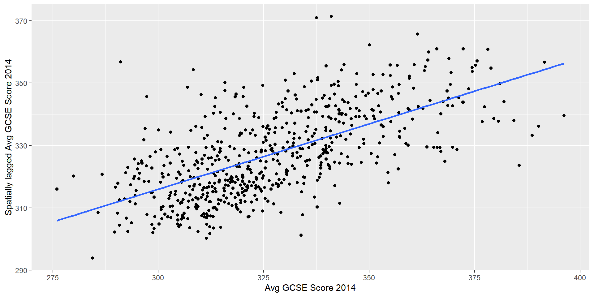
- If there is a linear correlation between the variable and its spatial lag (don’t ask me why the lag is the \(y\) variable in this case!), we can observe that values in near places do tend to cluster
Explaining Spatial Patterns
Having observed some spatial patterns in school exam performance in London, we might next want to explain these patterns, perhaps using another variable measured for the same spatial units.
Our own experience might tell us that missing class could negatively impact our ability to learn things in that class
Hypothesis: wards with higher rates of absence from school will tend to experience lower average exam grades
![]()

Explaining Spatial Patterns
(Intercept)
371.71500
unauthorised_absence_in_all_schools_percent_2013
-41.40264 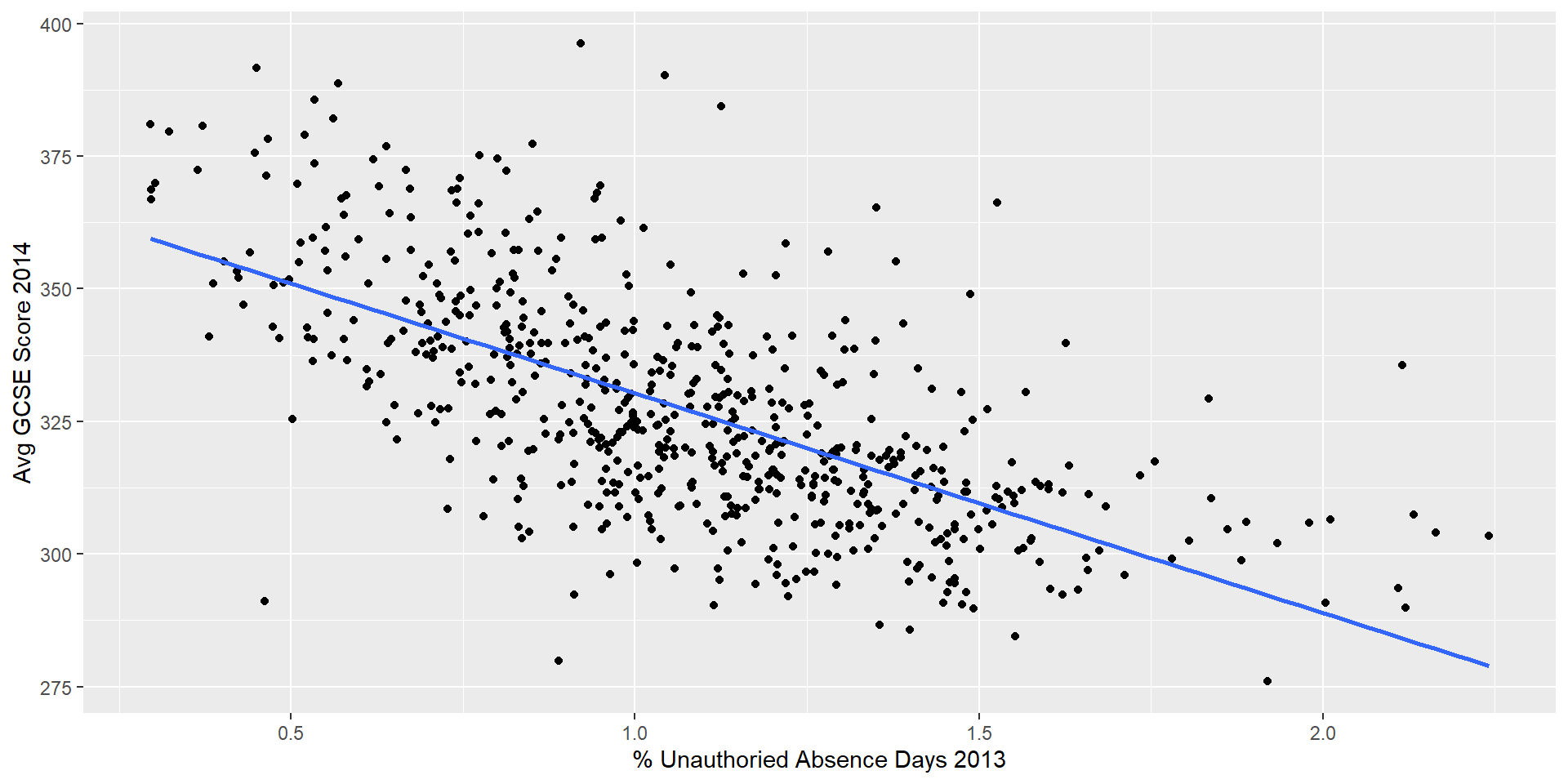
Taking the whole of London, it would appear that there is a moderately strong, negative relationship between missing school and exam performance
For every 1% of additional school days missed, we might expect a decrease of -41 points in GCSE score.
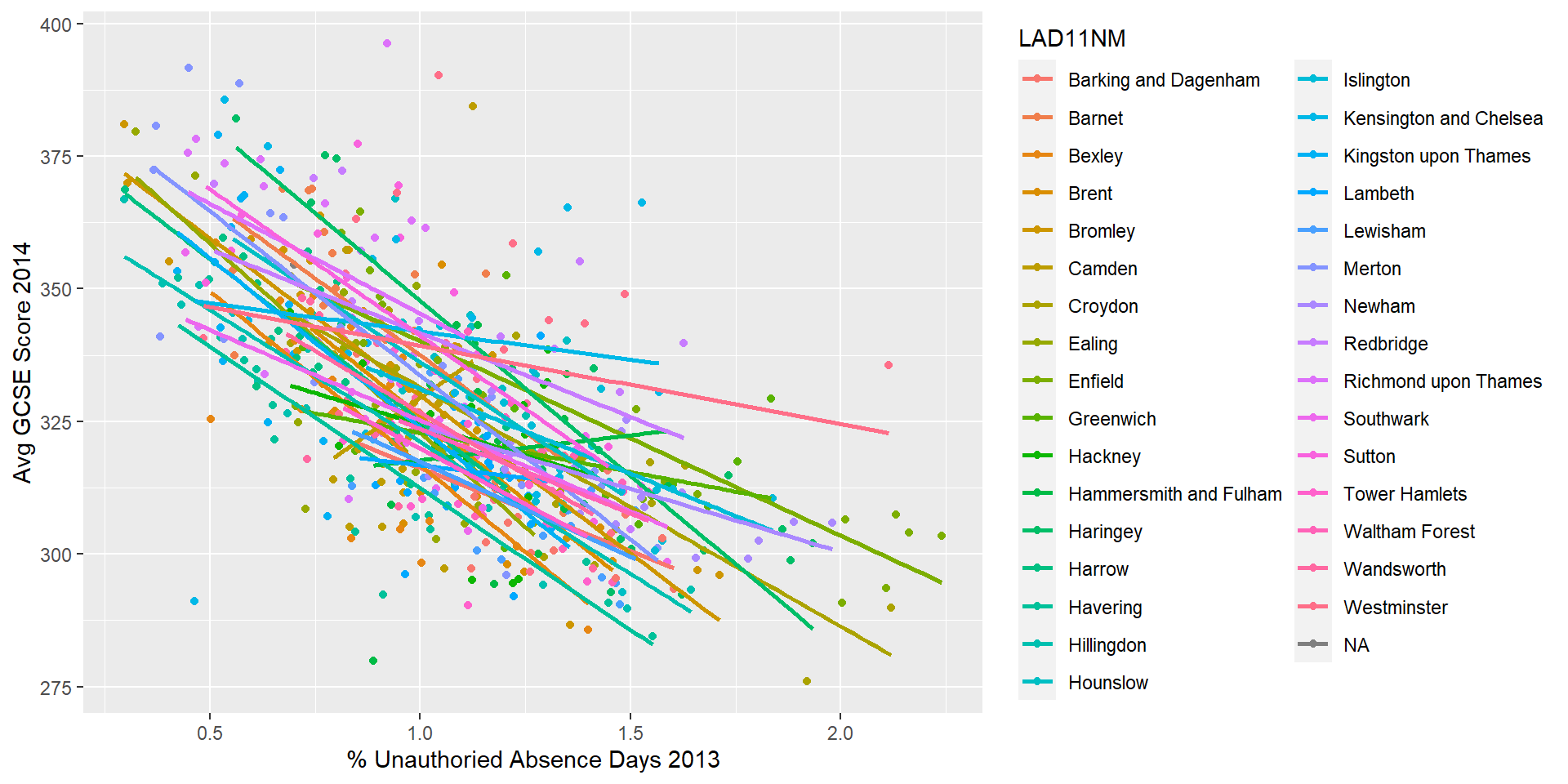
But does this relationship hold true across all wards in the city?
Dealing with Spatial Patterns - Spatial Non-Stationarity
One reason behind a clustering of residuals could be that the relationship between dependent and independent variables might not remain constant across space
In some parts of London, it could be that as unauthorised absence from school rises, exam grades also rise (as unlikely as that might be!).
Or, more plausibly, that in some parts of the city, absence has an even more pronounced negative effect than in others.
It’s also likely that the intercept values (the average value of GSCE rules, given no days of unauthorised absence) will be different in different parts of the city - some areas, on average, doing better than others
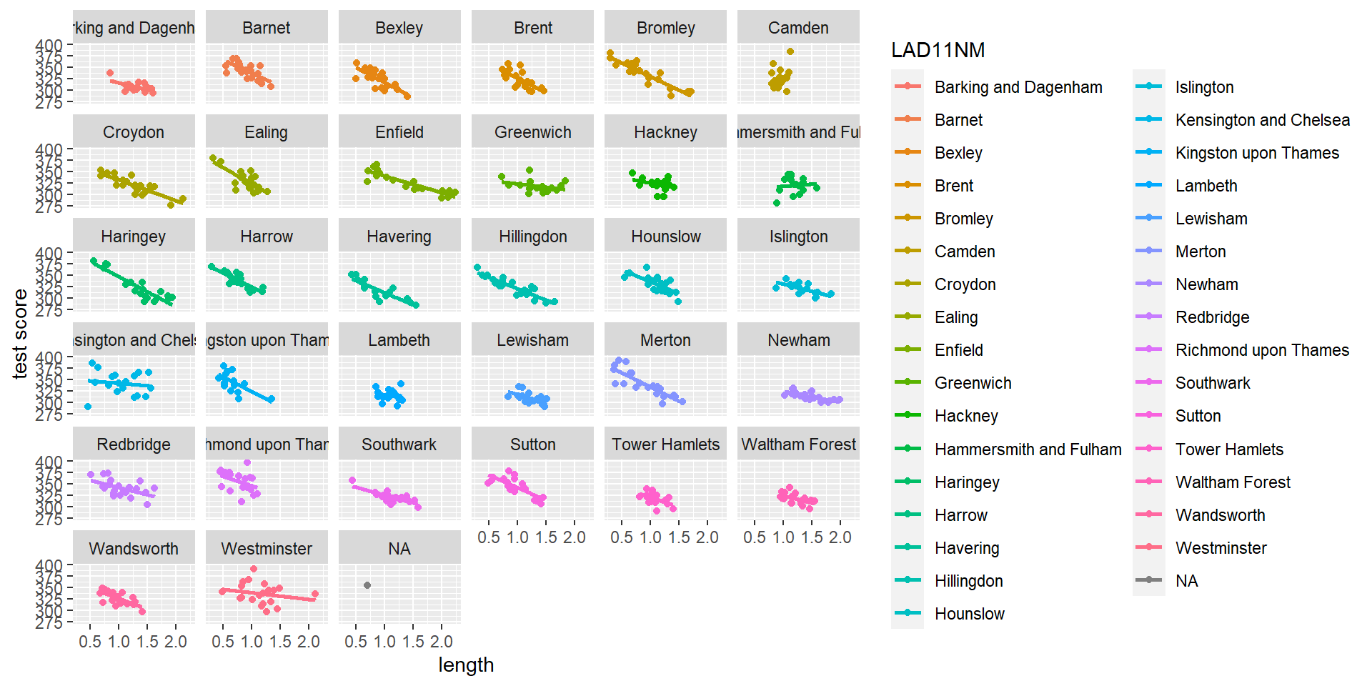
We can test for the presence of such phenomena by running a series of smaller, more localised regressions and comparing the coefficients that emerge
:focal(1205x459:1207x457)/origin-imgresizer.eurosport.com/2015/11/03/1725525-36508865-2560-1440.jpg)

Geographically Weighted Regression
GWR is a method for systematically running a series of localised regression analyses across a study area, collecting coefficients and other diagnostics for an independent variable in each zone of interest.
Something similar can be achieved through spatial sub-setting - i.e. running analyses for groups of zones within a higher level geography
Geographically Weighted Regression
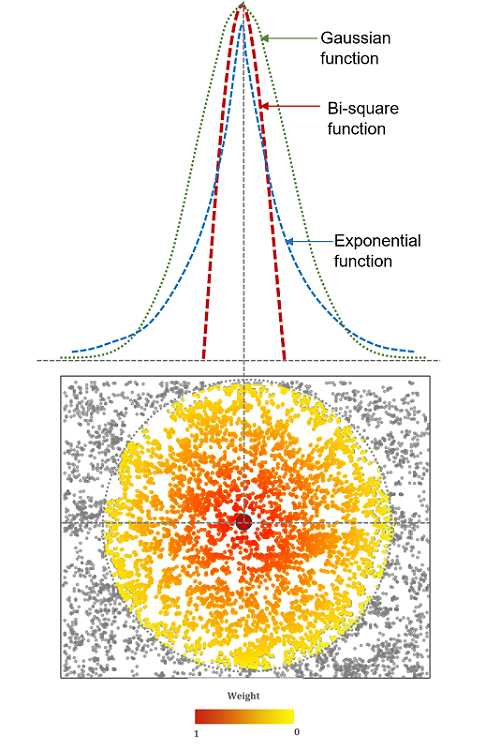
Geographically Weighted Regression
In a GWR analysis, kernel weighting functions of different bandwidths (diameters) and shapes are used to include and weight or exclude neighbouring observations
Adaptive weighting can be used to adjust the size of the kernel according to some threshold of observations
For every point in the dataset a regression is run including the values within the kernel (which, of course, can only be achieved effectively through understanding the coordinate reference system of the observations)
Scale and Shape - Modifiable Areal Units and Ecological Fallacies
Methods which accommodate space explicitly can help us better understand spatial phenomomena, but the arrangement of space can alter perceptions and the outcomes of analyses
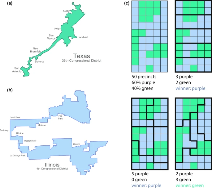
The Modifiable Areal Unit Problem (MAUP) - popularised in the 1980s by Stan Openshaw - describes issues that relate to the shape, scale and aggregation of underlying phenomenon to artificial spatial units
Politicians have known about the issues of scale and aggregation for a long time and have used it to their advantage
The practice of Gerrymandering is widespread wherever there is a first-past-the-post electoral system and has been used to manipulate vote counts to influence election outcomes
Conclusions
Knowing where something occurs underpins everything spatial data scientists do
Various conventions around how to locate something on the earth’s surface and store information about it have emerged
Near things are more related than distant things and being aware of this when analysing data with a spatial dimension is fundamental to carrying out a robust analysis
Accounting for spatial clustering in data can help analysts:
more correctly interpret relationships between variables
avoid making erroneous generalisations that do not apply in local contexts
be aware of potentially significant consequences in statistical outcomes that are the result of a particular arrangement of space